2022、FEDformer¶

约 6409 个字 3 张图片预计阅读时间 32 分钟

ICML2022、阿里达摩院

原文：《FEDformer: Frequency Enhanced Decomposed Transformer for Long-term Series Forecasting》

源码：https://github.com/DAMO-DI-ML/ICML2022-FEDformer

官方公众号：https://mp.weixin.qq.com/s/9doHueBCbsV7eUH2q3uv0A

关键词：

Autoformer 的改进
融合了transformer和经典信号处理方法：例如，利用傅立叶/小波变换将时域信息拆解为频域信息，让transformer更好地学习长时序中的依赖关系；FEDformer也能排除干扰，具有更好的鲁棒性。
专门设计周期趋势项分解模块：通过多次分解以降低输入输出的波动，进一步提升预测精度。
两个版本：傅里叶版本和小波变换版本（FEB-f 和 FEB-w）
专家混合分解机制

摘要¶

Although Transformer-based methods have significantly improved state-of-the-art results for long-term series forecasting, they are not only computationally expensive but more importantly, are unable to capture the global view of time series (e.g. overall trend). 尽管基于Transformer的方法显著提高了长期序列预测的最新结果，但它们不仅计算成本高，更重要的是，无法捕捉时间序列的全局视图（例如整体趋势）。

To address these problems, we propose to combine Transformer with the seasonal-trend decomposition method, in which the decomposition method captures the global profile of time series while Transformers capture more detailed structures.

为了解决这些问题，我们提出将Transformer与季节趋势分解方法结合起来，其中分解方法捕捉时间序列的全局轮廓，而Transformer捕捉更详细的结构。

To further enhance the performance of Transformer for longterm prediction, we exploit the fact that most time series tend to have a sparse representation in well-known basis such as Fourier transform, and develop a frequency enhanced Transformer.为了进一步提高Transformer在长期预测中的性能，我们利用大多数时间序列在诸如傅里叶变换等著名基底中具有稀疏表示这一事实，并开发了一种频率增强的Transformer。

频域增强

时间序列在傅里叶变换中具有稀疏性

Besides being more effective, the proposed method, termed as Frequency Enhanced Decomposed Transformer (FEDformer), is more efficient than standard Transformer with a linear complexity to the sequence length.

除了更有效之外，所提出的方法，称为频率增强分解Transformer（FEDformer），比标准Transformer更高效，其复杂度与序列长度呈线性关系。

复杂度呈现线性关系

Our empirical studies with six benchmark datasets show that compared with state-of-the-art methods, FEDformer can reduce prediction error by 14.8% and 22.6% for multivariate and univariate time series, respectively.

我们在六个基准数据集上的实证研究表明，与最先进的方法相比，FEDformer可以将多变量和单变量时间序列的预测误差分别降低14.8%和22.6%。

模型结构图¶

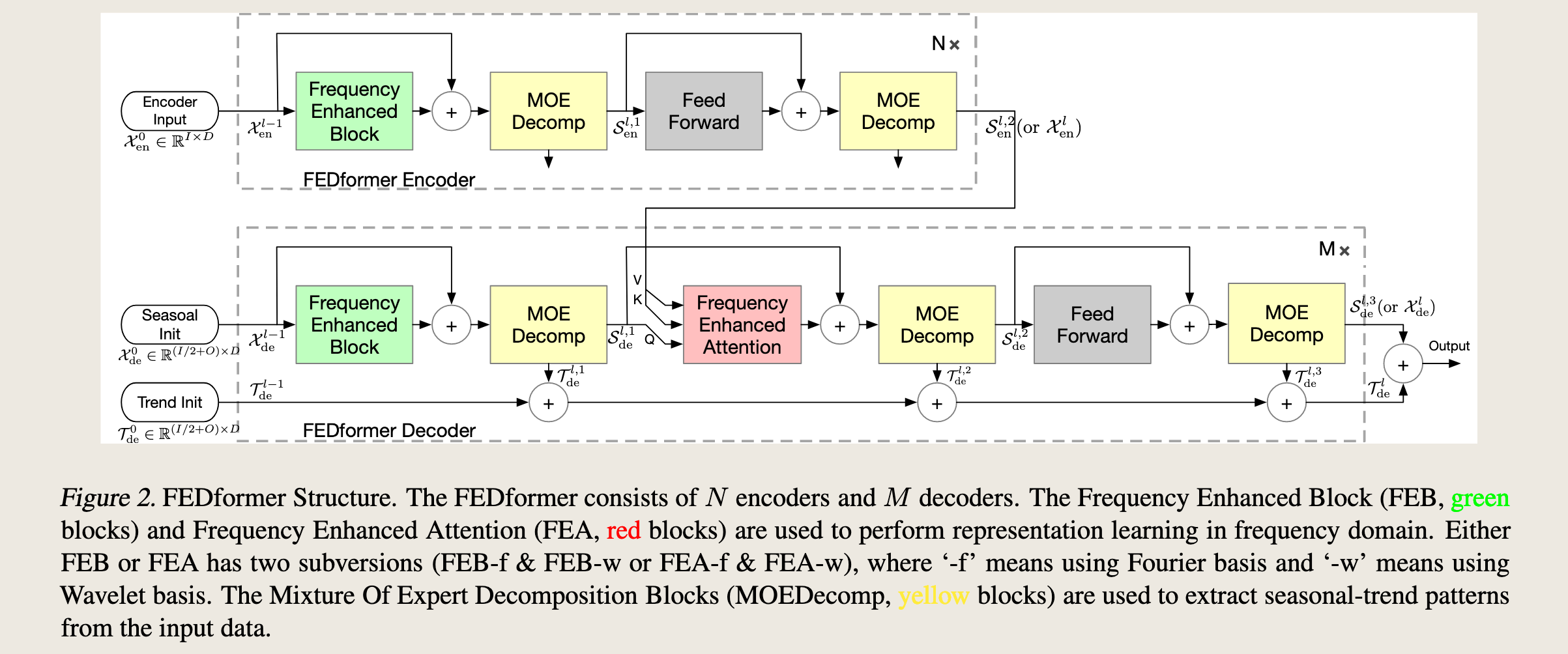
FEDformer（Frequency Enhanced Decomposed Transformer）的结构。FEDformer是一种用于长期时间序列预测的模型，它结合了频率增强块（Frequency Enhanced Block, FEB）和频率增强注意力（Frequency Enhanced Attention, FEA）

FEDformer Encoder

**Encoder Input $ \mathcal{X}_{en}^0 $ **: 输入数据，维度为 $\mathbb{R}^{ I \times D}$ 。
Frequency Enhanced Block (FEB): 绿色块，用于在频域中进行表示学习。FEB有两种变体：使用傅里叶基的FEB-f和使用小波基的FEB-w。
MOE Decomp (Mixture Of Expert Decomposition): 黄色块，用于从输入数据中提取季节性和趋势模式。
Feed Forward: 前馈网络，用于进一步处理数据。
$N×$: 表示编码器部分重复N次。

FEDformer Decoder

**Seasonal Init $\mathcal{X}_{de}^{l,0}$ **: 季节性初始化，维度为 $\mathbb{R}^{ (I/2+O) \times D}$ 。
**Trend Init $\mathcal{T}_{de}^0$ **: 趋势初始化，维度为 $\mathbb{R}^{(T/2+O) \times D}$ 。
Frequency Enhanced Block (FEB): 与编码器中的FEB相同，用于解码过程中的频域表示学习。
MOE Decomp: 与编码器中的MOE Decomp相同，用于解码过程中提取季节性和趋势模式。
Frequency Enhanced Attention (FEA): 红色块，用于在频域中进行注意力机制的表示学习。FEA也有两种变体：FEA-f和FEA-w。
$M×$: 表示解码器部分重复$M$次。
Output: 最终的预测输出。

符号说明：

$\mathcal{T}_{de}^{l,i}$ : 表示第 i 层解码器的趋势输出。
$\mathcal{S}_{de}^{l,i}$ : 表示第 i 层解码器的季节性输出。
$\mathcal{S}_{de}^{l,3}$ or $ \mathcal{X}_{de}^l$ : 最终的季节性输出或解码器输出。
看下标是编码器还是解码器；S 表示季节性成分，T 表示趋势性成分，因为真正的参数输入完全的白噪声，所以一般去除掉趋势性成分都归为季节性成分

总结

FEDformer通过结合频率增强块和频率增强注意力机制，在频域中进行有效的表示学习和注意力计算。同时，使用专家混合分解块（MOE Decomp）来提取输入数据的季节性和趋势模式。

3. Model Structure¶

In this section, we will introduce

(1) the overall structure of FEDformer, as shown in Figure 2,

(2) two subversion structures for signal process: one uses Fourier basis and the other uses Wavelet basis,

(3) the mixture of experts mechanism for seasonal-trend decomposition, and

(4) the complexity analysis of the proposed model.

在这一部分，我们将介绍：

FEDformer的整体结构，如图2所示；
两种信号处理的子版本结构：一种使用傅里叶基，另一种使用小波基；
用于季节性-趋势分解的专家混合机制；
所提出模型的复杂度分析。

3.1. FEDformer Framework¶

Preliminary Long-term time series forecasting is a sequence to sequence problem. We denote the input length as $I$ and output length as $O$. We denote $D$ as the hidden states of the series. The input of the encoder is a $I × D$ matrix and the decoder has $(I/2 + O) × D$ input.

符号说明：

输入序列 $I$
输出序列长度 $O$
隐藏层维度 $D$
编码器的输入 $I × D$
解码器的输入 $(I/2 + O) × D$ label length

FEDformer Structure Inspired by the seasonal-trend decomposition and distribution analysis as discussed in Section 1,

we renovate Transformer as a deep decomposition architecture as shown in Figure 2, including Frequency Enhanced Block (FEB), Frequency Enhanced Attention(FEA) connecting encoder and decoder, and the Mixture Of Experts Decomposition block (MOEDecomp).

The detailed description of FEB, FEA, and MOEDecomp blocks will be given in the following Section 3.2, 3.3, and 3.4 respectively.

贡献：FEB、FEA、MOED

频率增强模块
频率增强注意力
专家混合分解机制

Encoder

The encoder adopts a multilayer structure as:

$\mathcal{X}_{en}^{l} = \text{Encoder}(\mathcal{X}_{en}^{l-1})$

where $l ∈ {1, · · · , N }$ denotes the output of $l$-th encoder layer and $\mathcal{X}_{en}^{0} ∈ R^{I×D}$ is the embedded historical series.

编码器采用多层结构，每一层的输出表示为 $\mathcal{X}_{en}^{l}$，其中 $l$ 表示第 $l$ 层，$l \in {1, \dots, N}$。
初始输入 $ \mathcal{X}_{en}^{0}$ 是一个嵌入的历史序列，维度为 $ I \times D$。

The $\text{Encoder(·)}$ is formalized as

\[\begin{aligned} \mathcal{S}_ {\mathrm{en}}^{l,1}, & =\mathrm{MOEDecomp}(\mathrm{FEB}\left(\mathcal{X}_{\mathrm{en}}^{l-1}\right)+\mathcal{X}_{\mathrm{en}}^{l-1}), \\ \mathcal{S}_{\mathrm{en}}^{l,2},_{-} & =\mathrm{MOEDecomp}(\text{FeedForward}\left(\mathcal{S}_{\mathrm{en}}^{l,1}\right)+\mathcal{S}_{\mathrm{en}}^{l,1}),\quad(1) \\ \mathcal{X}_{\mathrm{en}}^{l} & =\mathcal{S}_{\mathsf{en}}^{l,2}, \end{aligned}\]

where $S_{en}^{l,i}, i ∈ {1, 2}$ represents the seasonal component after the $i$-th decomposition block in the $l$-th layer respectively.

首先，将输入 $ \mathcal{X}{en}^{l-1} $ 通过特征提取块（FEB）处理，然后加上输入本身，再进行混合专家分解（MOEDecomp），得到第一个季节性分量 $\mathcal{S} $。 }^{l,1
接着，将 $\mathcal{S}_{en}^{l,1} $ 通过前馈网络（FeedForward）处理，再加上 $ \mathcal{S}{en}^{l,1}$，再进行一次混合专家分解（MOEDecomp），得到第二个季节性分量 $\mathcal{S}_{en}^{l,2}$。
最终，将 $\mathcal{S}_{en}^{l,2}$ 作为当前层的输出 $\mathcal{X}_{en}^{l}$。

For FEB module, it has two different versions (FEB-f & FEB-w) which are implemented through Discrete Fourier transform (DFT) and Discrete Wavelet transform (DWT) mechanism respectively and can seamlessly replace the self-attention block.

FEB 模块有两种版本：

FEB-f：基于离散傅里叶变换（DFT）实现。
FEB-w：基于离散小波变换（DWT）实现。
这两种模块可以无缝替换传统的自注意力块。

总结：

基于多层结构的编码器，其中每一层通过特征提取块（FEB）和混合专家分解（MOEDecomp）模块来提取季节性分量。

FEB 模块有两种实现方式（基于 DFT 和 DWT），可以替代传统的自注意力机制。

The decoder also adopts a multilayer structure as:

$\mathcal{X}_{de}^{l-1}, \mathcal{T}_{de}^{l-1} = \mathrm{Decoder}(\mathcal{X}^{l−1}_{de} , \mathcal{T}_{de}^{l−1} )$,

where $l ∈ {1, · · · , M }$ denotes the output of $l$-th decoder layer.

The $\mathrm{Decoder}(·)$ is formalized as

\[\begin{aligned} \mathcal{S}_{\mathrm{de}}^{l,1},\mathcal{T}_{\mathrm{de}}^{l,1} & =\mathrm{MOEDecomp}\left(\mathrm{FEB}\left(\mathcal{X}_{\mathrm{de}}^{l-1}\right)+\mathcal{X}_{\mathrm{de}}^{l-1}\right), \\ \mathcal{S}_{\mathrm{de}}^{l,2},\mathcal{T}_{\mathrm{de}}^{l,2} & =\mathrm{MOEDecomp}\left(\mathrm{FEA}\left(\mathcal{S}_{\mathrm{de}}^{l,1},\mathcal{X}_{\mathrm{en}}^N\right)+\mathcal{S}_{\mathrm{de}}^{l,1}\right), \\ \mathcal{S}_{\mathrm{de}}^{l,3},\mathcal{T}_{\mathrm{de}}^{l,3} & =\mathrm{MOEDecomp}\left(\text{FeedForward}\left(\mathcal{S}_{\mathrm{de}}^{l,2}\right)+\mathcal{S}_{\mathrm{de}}^{l,2}\right), \\ \mathcal{X}_{\mathrm{de}}^l & =\mathcal{S}_{\mathsf{de}}^{l,3}, \\ \mathcal{T}_{\mathrm{de}}^l & =\mathcal{T}_{\mathrm{de}}^{l-1}+\mathcal{W}_{l,1}\cdot\mathcal{T}_{\mathrm{de}}^{l,1}+\mathcal{W}_{l,2}\cdot\mathcal{T}_{\mathrm{de}}^{l,2}+\mathcal{W}_{l,3}\cdot\mathcal{T}_{\mathrm{de}}^{l,3}, \end{aligned}\]

where $\mathcal{S}_{de}^{l,i} , \mathcal{T}_{de}^{l,i} , i ∈ {1, 2, 3}$ represent the seasonal and trend component after the $i$-th decomposition block in the $l$-th layer respectively. 第 $l$ 层第 $i$ 个分解块

$ W_{l,i}, i ∈ {1, 2, 3}$ represents the projector for the $i$-th extracted trend $T^{l,i}_{de}$ .

与编码器类似，但增加了趋势（Trend）分量的处理，并引入了特征提取模块（FEA）
解码器采用多层结构，每一层的输出表示为 $\mathcal{S}_{de}^{l,i}$ 和 $\mathcal{T}_{de}^{l,i}$，其中 $l$ 表示第 $l$ 层，$(l \in {1, \dots, M})$
$\mathcal{X}_{de}^{l}$ 表示解码器的输出，而 $\mathcal{T}_{de}^{l}$ 表示趋势分量。
第一步：将输入 $\mathcal{X}_{de}^{l-1}$ 通过特征提取块（FEB）处理，然后加上输入本身，再进行混合专家分解（MOEDecomp），得到第一个季节性分量 $\mathcal{S}_{de}^{l,1}$ 和第一个趋势分量 $\mathcal{T}_{de}^{l,1}$。
第二步：将 $\mathcal{S}_{de}^{l,1}$ 和编码器的输出 $\mathcal{X}_{en}^N$ 通过特征提取模块（FEA）处理，再加上 $\mathcal{S}_{de}^{l,1}$，再进行一次混合专家分解（MOEDecomp），得到第二个季节性分量 $\mathcal{S}_{de}^{l,2}$ 和第二个趋势分量 $\mathcal{T}_{de}^{l,2}$。
第三步：将 $\mathcal{S}_{de}^{l,2}$ 通过前馈网络（FeedForward）处理，再加上 $\mathcal{S}_{de}^{l,2}$，再进行一次混合专家分解（MOEDecomp），得到第三个季节性分量 $\mathcal{S}_{de}^{l,3}$ 和第三个趋势分量 $\mathcal{T}_{de}^{l,3}$。
最终输出：将 $\mathcal{S}_{de}^{l,3}$ 作为当前层的输出 $\mathcal{X}_{de}^{l}$。
趋势分量更新：将 $\mathcal{T}_{de}^{l}$ 更新为 $\mathcal{T}_{de}^{l-1}$ 加上三个趋势分量的加权和，权重分别为 $\mathcal{W}_{l,1}$、$\mathcal{W}_{l,2}$ 和 $\mathcal{W}_{l,3}$。

Similar to FEB, FEA has two different versions (FEA-f & FEA-w) which are implemented through DFT and DWT projection respectively with attention design, and can replace the cross-attention block.

FEA 模块有两种版本：

FEA-f：基于离散傅里叶变换（DFT）实现。
FEA-w：基于离散小波变换（DWT）实现。

这两种模块都设计了注意力机制，可以无缝替换传统的交叉注意力块。

解码器的多层结构：

每一层通过特征提取块（FEB）、特征提取模块（FEA）和混合专家分解（MOEDecomp）来提取季节性和趋势分量。

解码器的输出包括季节性分量和趋势分量，趋势分量通过加权和进行更新。

FEA 模块有两种实现方式（基于 DFT 和 DWT），并设计了注意力机制，可以替代传统的交叉注意力块。

The final prediction is the sum of the two refined decomposed components as $\mathcal{W}_S · \mathcal{X}_{de}^M + \mathcal{T}_{de}^M$ , where $\mathcal{W}_S$ is to project the deep transformed seasonal component $\mathcal{X}_{de}^M$ to the target dimension.

最终预测是两个经过细化的分解分量的和，表示为 $\mathcal{W}_S \cdot \mathcal{X}_{de}^M + \mathcal{T}_{de}^M$，其中 $\mathcal{W}_S$ 用于将深度变换后的季节性分量 $\mathcal{X}_{de}^M$ 投影到目标维度。

3.2. Fourier Enhanced Structure¶

Discrete Fourier Transform (DFT)

The proposed Fourier Enhanced Structures use discrete Fourier transform (DFT). Let $\mathcal{F}$ denotes the Fourier transform and $\mathcal{F}^{-1}$ denotes the inverse Fourier transform.

傅里叶变换和逆变换

令 $\mathcal{F}$ 表示傅里叶变换，$\mathcal{F}^{-1}$ 表示逆傅里叶变换。

Given a sequence of real numbers $x_n$ in time domain, where $n = 1, 2...N$ . DFT is defined as $X_l = \sum_{n=0}^{N-1} x_ne^{−i\omega ln}$, where $i$ is the imaginary unit and $X_l, l = 1, 2...L$ is a sequence of complex numbers in the frequency domain. Similarly, the inverse DFT is defined as $x_n = \sum_{n=0}^{N-1} X_l e^{i\omega ln}$ .

给定一个实数序列 $x_n$ 在时域中，其中 $n = 1, 2, \ldots, N$。DFT 定义为： $$ X_l = \sum_{n=0}^{N-1} x_n e^{-i\omega ln} $$ 其中 $i$ 是虚数单位，$X_l, l = 1, 2, \ldots, L$ 是一个在频域中的复数序列。

类似地，逆 DFT 定义为： $$ x_n = \sum_{l=0}^{N-1} X_l e^{i\omega ln} $$ The complexity of DFT is $O(N^2)$. With fast Fourier transform (FFT), the computation complexity can be reduced to $O(N log N )$. Here a random subset of the Fourier basis is used and the scale of the subset is bounded by a scalar. When we choose the mode index before DFT and reverse DFT operations, the computation complexity can be further reduced to $O(N )$.

DFT 的计算复杂度是 $O(N ^2)$。
使用快速傅里叶变换（FFT），计算复杂度可以降低到 $O(N \log N)$。
在这里，使用了傅里叶基的一个随机子集，并且子集的规模由一个标量限制。当在 DFT 和逆 DFT 操作之前选择模式索引时，计算复杂度可以进一步降低到 $O(N)$。

Frequency Enhanced Block with Fourier Transform (FEB-f) . The FEB-f is used in both encoder and decoder as shown in Figure 2.

“频率增强块”（Frequency Enhanced Block，简称FEB-f）使用傅里叶变换（Fourier Transform）来处理数据。FEB-f 被用于编码器和解码器中。

The input ($x \in \mathbb{R}^{N \times D}$) of the FEB-f block is first linearly projected with $w \in \mathbb{R}^{D \times D}$, so $q = x \cdot w$.

输入处理：输入数据 $x \in \mathbb{R}^{N \times D}$ 首先通过一个线性投影 $w \in \mathbb{R}^{D \times D}$ 进行变换，得到 $q = x \cdot w$。

Then $q$ is converted from the time domain to the frequency domain. The Fourier transform of $q$ is denoted as $Q \in \mathbb{C}^{N \times D}$.

傅里叶变换：将 $q$ 从时域转换到频域，得到 $Q \in \mathbb{C}^{N \times D}$。

In frequency domain, only the randomly selected $M$ modes are kept so we use a select operator as

选择操作：在频域中，只保留随机选择的 $M$ 个模式，使用选择操作 $\text{Select}(Q) = \text{Select}(\mathcal{F}(q))$，得到 $\tilde{Q} \in \mathbb{C}^{M \times D}$，其中 $M \ll N$。 $$ \tilde{Q} = \text{Select}(Q) = \text{Select}(\mathcal{F}(q)), $$

where $\tilde{Q} \in \mathbb{C}^{M \times D}$ and $M \ll N$.

Then, the FEB-f is defined as $$ \text{FEB-f}(q) = \mathcal{F}^{-1}(\text{Padding}(\tilde{Q} \odot R)), $$

where $R \in \mathbb{C}^{D \times D \times M}$ is a parameterized kernel initialized randomly.

FEB-f 定义：FEB-f 的定义为 $\text{FEB-f}(q) = \mathcal{F}^{-1}(\text{Padding}(\tilde{Q} \odot R))$，其中 $R \in \mathbb{C}^{D \times D \times M}$ 是一个随机初始化的参数化核。

Let $Y = Q \odot C$, with $Y \in \mathbb{C}^{M \times D}$. The production operator $\odot$ is defined as: $Y_{m,d_o} = \sum_{d_i=0}^{D} Q_{m,d_i} \cdot R_{d_i,d_o,m}$, where $d_i = 1, 2...D$ is the input channel and $d_o = 1, 2...D$ is the output channel.

生产操作：定义了生产操作 $\odot$，用于计算 $Y = Q \odot C$，其中 $Y \in \mathbb{C}^{M \times D}$。生产操作的具体定义为 $Y_{m,d_o} = \sum_{d_i=0}^{D} Q_{m,d_i} \cdot R_{d_i,d_o,m}$，其中 $d_i$ 和 $d_o$ 分别表示输入和输出通道。

The result of $Q \odot R$ is then zero-padded to $\mathbb{C}^{N \times D}$ before performing inverse Fourier transform back to the time domain. The structure is shown in Figure 3.

逆傅里叶变换：$Q \odot R$ 的结果首先进行零填充到 $\mathbb{C}^{N \times D}$，然后执行逆傅里叶变换回到时域。

涉及到频域的论文都，好难啊啊啊啊ε＝ε＝ε＝(#>д<)ﾉ

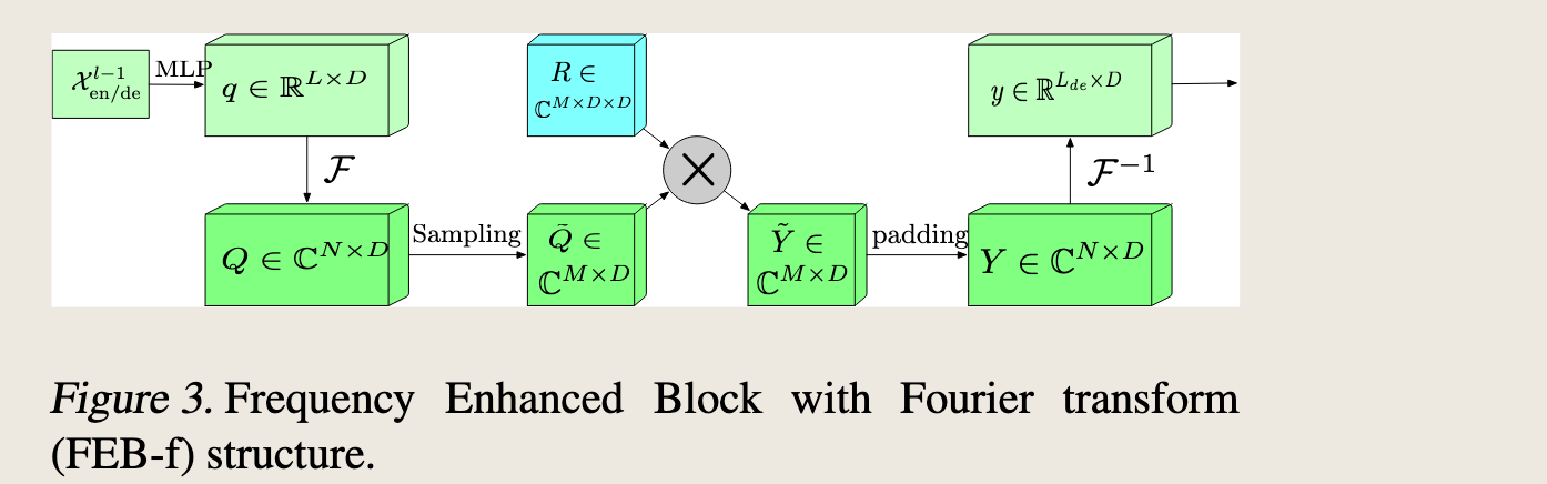
图 3 展示了一个使用傅里叶变换（FEB-f）的频率增强块（Frequency Enhanced Block）的结构：

输入：输入数据 $x^{l-1}_{en/de}$ 经过多层感知机（MLP）处理，得到 $q \in \mathbb{R}^{L \times D}$。
傅里叶变换：对 $q$ 进行傅里叶变换 $\mathcal{F}$，得到频域表示 $Q \in \mathbb{C}^{N \times D}$。
采样：在频域中，对 $Q$ 进行采样，保留 $M$ 个模式，得到 $\tilde{Q} \in \mathbb{C}^{M \times D}$。
参数化核：使用一个参数化核 $R \in \mathbb{C}^{M \times D \times D}$，该核是随机初始化的。
乘法操作：将 $\tilde{Q}$ 和 $R$ 进行逐元素乘法（Hadamard 乘积），得到 $\tilde{Y} \in \mathbb{C}^{M \times D}$。
填充：将 $\tilde{Y}$ 进行零填充（padding），使其维度恢复到 $Y \in \mathbb{C}^{N \times D}$。
逆傅里叶变换：对填充后的 $Y$ 进行逆傅里叶变换 $\mathcal{F}^{-1}$，得到时域表示 $y \in \mathbb{R}^{L_{de} \times D}$。

总结来说，这个频率增强块通过傅里叶变换将输入数据转换到频域，然后选择性地保留重要的频率模式，再通过参数化核进行处理，最后通过逆傅里叶变换将结果转换回时域。这种结构可以有效地提取和处理频率信息，从而增强模型的性能。

Frequency Enhanced Attention with Fourier Transform (FEA-f)

We use the expression of the canonical transformer.

The input: queries, keys, values are denoted as $q \in \mathbb{R}^{L \times D}$, $k \in \mathbb{R}^{L \times D}$, $v \in \mathbb{R}^{L \times D}$.

输入：输入包括查询（queries）、键（keys）和值（values），分别表示为 $q \in \mathbb{R}^{L \times D}$，$k \in \mathbb{R}^{L \times D}$，$v \in \mathbb{R}^{L \times D}$。

In cross-attention, the queries come from the decoder and can be obtained by $q = x_{en} \cdot w_q$, where $w_q \in \mathbb{R}^{D \times D}$.

The keys and values are from the encoder and can be obtained by $k = x_{de} \cdot w_k$ and $v = x_{de} \cdot w_v$, where $w_k, w_v \in \mathbb{R}^{D \times D}$.

Formally, the canonical attention can be written as $$ \text{Atten}(q, k, v) = \text{Softmax}\left(\frac{q k^\top}{\sqrt{d_q}}\right) v. $$

传统注意力机制：传统注意力机制可以表示为 $$ \text{Atten}(q, k, v) = \text{Softmax}\left(\frac{q k^\top}{\sqrt{d_q}}\right) v. $$ FEA-f 机制

In FEA-f, we convert the queries, keys, and values with Fourier Transform and perform a similar attention mechanism in the frequency domain, by randomly selecting $M$ modes. We denote the selected version after Fourier Transform as $\tilde{Q} \in \mathbb{C}^{M \times D}$, $\tilde{K} \in \mathbb{C}^{M \times D}$, $\tilde{V} \in \mathbb{C}^{M \times D}$.

首先，对查询、键和值进行傅里叶变换，并在频域中随机选择 $M$ 个模式，得到 $\tilde{Q} \in \mathbb{C}^{M \times D}$，$\tilde{K} \in \mathbb{C}^{M \times D}$，$\tilde{V} \in \mathbb{C}^{M \times D}$。

The FEA-f is defined as $$ \tilde{Q} = \text{Select}(\mathcal{F}(q)) $$

\[ \tilde{K} = \text{Select}(\mathcal{F}(k)) \]

\[ \tilde{V} = \text{Select}(\mathcal{F}(v)) \]

\[ \text{FEA-f}(q, k, v) = \mathcal{F}^{-1}(\text{Padding}(\sigma(\tilde{Q} \cdot \tilde{K}^\top) \cdot \tilde{V})), \]

where $\sigma$ is the activation function.

然后，定义 FEA-f 为 $$ \text{FEA-f}(q, k, v) = \mathcal{F}^{-1}(\text{Padding}(\sigma(\tilde{Q} \cdot \tilde{K}^\top) \cdot \tilde{V})), $$ We use softmax or tanh for activation, since their converging performance differs in different data sets. Let $Y = \sigma(\tilde{Q} \cdot \tilde{K}^\top) \cdot \tilde{V}$,

其中 $\sigma$ 是激活函数，可以使用 softmax 或 tanh，因为它们在不同数据集上的收敛性能不同。

激活函数：激活函数 $\sigma$ 用于计算 $\tilde{Q} \cdot \tilde{K}^\top$ 和 $\tilde{V}$ 的逐元素乘积，得到 $Y = \sigma(\tilde{Q} \cdot \tilde{K}^\top) \cdot \tilde{V}$，其中 $Y \in \mathbb{C}^{M \times D}$。

and $Y \in \mathbb{C}^{M \times D}$ needs to be zero-padded to $\mathbb{C}^{L \times D}$ before performing inverse Fourier transform. The FEA-f structure is shown in Figure 4.

逆傅里叶变换：将 $Y$ 进行零填充到 $\mathbb{C}^{L \times D}$，然后进行逆傅里叶变换，得到最终的输出。

3.3. Wavelet Enhanced Structure¶

Discrete Wavelet Transform (DWT) While the Fourier transform creates a representation of the signal in the frequency domain, the Wavelet transform creates a representation in both the frequency and time domain, allowing efficient access of localized information of the signal.

Fourier 变换在频域中创建信号的表示，而小波变换则在频域和时域中同时创建信号的表示，允许高效访问信号的局部信息。

The multiwavelet transform synergizes the advantages of orthogonal polynomials as well as wavelets.

多小波变换结合了正交多项式和小波的优势。

For a given $f(x)$, the multiwavelet coefficients at the scale $n$ can be defined as $s_l^n = \left[\left\langle f, \phi_{il}^n \right\rangle_{\mu_n}\right]_{i=0}^{k-1}$, $d_l^n = \left[\left\langle f, \psi_{il}^n \right\rangle_{\mu_n}\right]_{i=0}^{k-1}$, respectively, w.r.t. measure $\mu_n$ with $s_l^n, d_l^n \in \mathbb{R}^{k \times 2^n}$. $\phi_{il}^n$ are wavelet orthonormal basis of piecewise polynomials.

对于给定的函数 $f(x)$，尺度为 $n$ 的多小波系数可以定义为 $s_l^n = \left[\left\langle f, \phi_{il}^n \right\rangle_{\mu_n}\right]_{i=0}^{k-1}$，$d_l^n = \left[\left\langle f, \psi_{il}^n \right\rangle_{\mu_n}\right]_{i=0}^{k-1}$，分别对应于测度 $\mu_n$，其中 $s_l^n, d_l^n \in \mathbb{R}^{k \times 2^n}$。$\phi_{il}^n$ 是分段多项式的小波正交基。

对于给定的函数 $f(x)$，在尺度 $n$ 下的多小波系数可以定义为：
尺度系数 $s_l^n = \left[\left\langle f, \phi_{il}^n \right\rangle_{\mu_n}\right]_{i=0}^{k-1}$
细节系数 $d_l^n = \left[\left\langle f, \psi_{il}^n \right\rangle_{\mu_n}\right]_{i=0}^{k-1}$
这里，$\left\langle f, \phi_{il}^n \right\rangle_{\mu_n}$ 和 $\left\langle f, \psi_{il}^n \right\rangle_{\mu_n}$ 分别表示函数 $f$ 与尺度函数 $\phi_{il}^n$ 和小波函数 $\psi_{il}^n$ 的内积，相对于测度 $\mu_n$。
$s_l^n, d_l^n \in \mathbb{R}^{k \times 2^n}$ 表示这些系数的维度。
$\phi_{il}^n$ 是分段多项式的小波正交基函数，这些基函数用于构建小波变换。

The decomposition/reconstruction across scales is defined as

尺度分解和重建结构定义如下：

\[ \begin{aligned} \mathbf{s}_l^n &= H^{(0)} \mathbf{s}_{2l}^{n+1} + H^{(1)} \mathbf{s}_{2l+1}^{n+1}, \\ \mathbf{s}_{2l}^{n+1} &= \Sigma^{(0)} \left( H^{(0)T} \mathbf{s}_l^n + G^{(0)T} \mathbf{d}_l^n \right), \\ \mathbf{d}_l^n &= G^{(0)} \mathbf{s}_{2l}^{n+1} + H^{(1)} \mathbf{s}_{2l+1}^{n+1}, \\ \mathbf{s}_{2l+1}^{n+1} &= \Sigma^{(1)} \left( H^{(1)T} \mathbf{s}_l^n + G^{(1)T} \mathbf{d}_l^n \right), \end{aligned} \]

where $(H^{(0)}, H^{(1)}, G^{(0)}, G^{(1)})$ are linear coefficients for multiwavelet decomposition filters.

给出了多小波分解的一组公式，涉及到尺度系数 $\mathbf{s}_l^n$ 和细节系数 $\mathbf{d}_l^n$ 的计算。
使用了固定的线性系数矩阵 $H^{(0)}$, $H^{(1)}$, $G^{(0)}$, $G^{(1)}$ 来表示多小波分解滤波器。

They are fixed matrices used for wavelet decomposition.

The multiwavelet representation of a signal can be obtained by the tensor product of multiscale and multiwavelet basis.

信号的多小波表示可以通过多尺度和多小波基的张量积获得。

Note that the basis at various scales are coupled by the tensor product, so we need to untangle it. Inspired by (Gupta et al., 2021), we adapt a non-standard wavelet representation to reduce the model complexity.

请注意，不同尺度的基通过张量积耦合在一起，因此我们需要将其解耦。受 Gupta 等人（2021）的启发，我们采用了一种非标准的小波表示来降低模型复杂度。

For a map function $F(x) = x'$, the map under multiwavelet domain can be written as $$ U_{dl}^n = A_n d_l^n + B_n s_l^n, \quad U_{sl}^n = C_n d_l^n, \quad U_{sl}^L = \bar{F} s_l^L, $$

where $(U_{sl}^n, U_{dl}^n, s_l^n, d_l^n)$ are the multiscale, multiwavelet coefficients, $L$ is the coarsest scale under recursive decomposition, and $A_n, B_n, C_n$ are three independent FEB-f blocks modules used for processing different signal during decomposition and reconstruction.

对于映射函数 $F(x) = x'$，在多小波域中的映射可以表示为： $$ U_{dl}^n = A_n d_l^n + B_n s_l^n, \quad U_{sl}^n = C_n d_l^n, \quad U_{sl}^L = \bar{F} s_l^L, $$

其中 $(U_{sl}^n, U_{dl}^n, s_l^n, d_l^n)$ 是多尺度、多小波系数，$L$ 是递归分解下的最粗糙尺度，$A_n, B_n, C_n$ 是三个独立的 FEB-f 块模块，用于在分解和重构过程中处理不同的信号。

Here $\bar{F}$ is a single-layer of perceptrons which processes the remaining coarsest signal after $L$ decomposed steps. More designed detail is described in Appendix D.

这里 $\bar{F}$ 是一个单层感知器，用于处理 $L$ 次分解步骤后剩余的最粗糙信号。更多设计细节在附录 D 中描述。

原文如下：

Frequency Enhanced Block with Wavelet Transform (FEB-w)

The overall FEB-w architecture is shown in Figure 5.

频率增强块与小波变换（FEB-w）的整体 FEB-w 架构如图 5 所示。

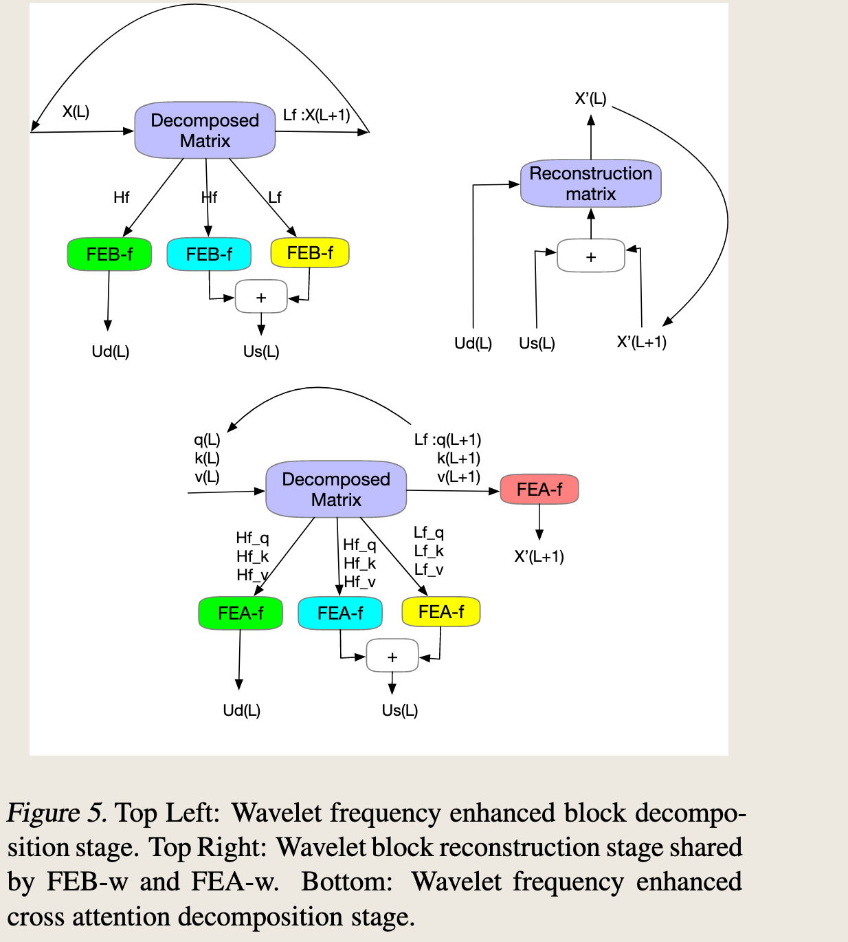
It differs from FEB-f in the recursive mechanism: the input is decomposed into 3 parts recursively and operates individually.

它与 FEB-f 在递归机制上有所不同：输入被递归地分解为 3 个部分并分别进行操作。

For the wavelet decomposition part, we implement the fixed Legendre wavelets basis decomposition matrix.

对于小波分解部分，我们实现了固定的勒让德小波基分解矩阵。

Three FEB-f modules are used to process the resulting high-frequency part, low-frequency part, and remaining part from wavelet decomposition respectively.

三个 FEB-f 模块分别用于处理小波分解得到的高频部分、低频部分和剩余部分。

For each cycle $L$, it produces a processed high-frequency tensor $Ud(L)$, a processed low-frequency frequency tensor $Us(L)$, and the raw low-frequency tensor $X(L+1)$.

对于每个周期 $L$，它生成一个处理过的高频张量 $Ud(L)$，一个处理过的低频频率张量$Us(L)$，以及原始的低频张量 $X(L+1)$。

This is a ladder-down approach, and the decomposition stage performs the decimation of the signal by a factor of $1/2$, running for a maximum of $L$ cycles, where $L < \log_2(M)$ for a given input sequence of size $M$.

这是一种逐级下降的方法，分解阶段通过 $1/2$ 的因子对信号进行降采样，最多运行 $L$ 个周期，其中对于给定大小为 $M$ 的输入序列，$L < \log_2(M)$。

In practice, $L$ is set as a fixed argument parameter. The three sets of FEB-f blocks are shared during different decomposition cycles $L$.

在实践中，$L$ 被设定为一个固定的参数。在不同的分解周期 $L$ 中，三组 FEB-f 模块是共享的。

For the wavelet reconstruction part, we recursively build up our output tensor as well. 对于小波重构部分，我们同样递归地构建输出张量。

For each cycle $L$, we combine $X(L+1)$, $Us(L)$, and $Ud(L)$ produced from the decomposition part and produce $X(L)$ for the next reconstruction cycle. For each cycle, the length dimension of the signal tensor is increased by 2 times.

对于每个周期 $L$，我们结合从分解部分产生的 $X(L+1)$、$Us(L)$ 和 $Ud(L)$，并生成下一个重构周期的 $X(L)$。对于每个周期，信号张量的长度维度增加两倍。

在信号处理过程中，$Us(L)$ 表示第 $L$ 层的尺度系数，而 $X(L+1)$ 代表原始的低频张量。该方法采用逐级下降策略，其中分解阶段将信号的采样率降低为原来的一半，这一过程最多重复 $L$ 次。这里，$L$ 的值取决于输入序列的大小 $M$，并且满足 $L < \log_2(M)$。在实际操作中，$L$ 作为一个固定参数进行设置。在不同的分解周期中，三组 FEB-f 模块会被重复使用。在小波重构阶段，我们递归地构建最终的输出张量。具体来说，在每个周期 $L$，我们将由分解阶段生成的 $X(L+1)$、$Us(L)$ 和 $Ud(L)$ 结合起来，以产生用于下一个重构周期的 $X(L)$。在每个周期内，信号张量的长度维度都会翻倍。

原文识别如下：

3.4. Mixture of Experts for Seasonal-Trend Decomposition¶

3.4 专家混合模型在季节-趋势分解中的应用

Because of the commonly observed complex periodic pattern coupled with the trend component on real-world data, extracting the trend can be hard with fixed window average pooling.

由于在实际数据中常见的复杂周期模式与趋势成分相结合，使用固定窗口平均池化提取趋势可能较为困难。

To overcome such a problem, we design a Mixture Of Experts Decomposition block (MOEDecomp). It contains a set of average filters with different sizes to extract multiple trend components from the input signal and a set of data-dependent weights for combining them as the final trend. Formally, we have

为了解决这一问题，我们设计了一种专家混合分解模块（MOEDecomp）。该模块包含一组不同尺寸的平均滤波器，用于从输入信号中提取多个趋势成分，以及一组数据依赖的权重，用于将这些成分组合成最终趋势。形式上，我们有： $$ X_{\text{trend}} = \text{Softmax}(L(x)) * (F(x)), $$

where $F(\cdot)$ is a set of average pooling filters and $\text{Softmax}(L(x))$ is the weights for mixing these extracted trends.

\[ X_{\text{trend}} = \text{Softmax}(L(x)) * (F(x)), \]

其中 $F(\cdot)$ 表示一组平均池化滤波器，而 $\text{Softmax}(L(x))$ 表示用于混合这些提取出的趋势的权重。

add_circle2025-04-13 13:01:53update2025-04-13 22:00:41