2023、WITRAN¶

约 6196 个字 8 张图片预计阅读时间 31 分钟

NeurIPS 2023

论文：https://openreview.net/pdf?id=y08bkEtNBK

源码：https://github.com/Water2sea/WITRAN/tree/main

实验室公众号：https://mp.weixin.qq.com/s/kkNEpZOAn9MFUGg5P9ZfXQ

摘要¶

Capturing semantic information is crucial for accurate long-range time series forecasting, which involves modeling global and local correlations, as well as discovering long- and short-term repetitive patterns. Previous works have partially addressed these issues separately, but have not been able to address all of them simultaneously.

捕获语义信息对于准确的长期时间序列预测至关重要，这涉及到对全局和局部相关性的建模，以及发现长期和短期的重复模式。以往的研究分别部分解决了这些问题，但尚未能够同时解决所有这些问题。

Meanwhile, their time and memory complexities are still not sufficiently low for long-range forecasting.

To address the challenge of capturing different types of semantic information, we propose a novel Water-wave Information Transmission (WIT) framework.

This framework captures both long- and short-term repetitive patterns through bi-granular information transmission.

同时，它们在长期预测中的时间复杂度和内存复杂度仍然不够低。为了应对捕获不同类型的语义信息的挑战，我们提出了一种新颖的水波信息传输（WIT）框架。该框架通过双粒度信息传输捕获长期和短期的重复模式。

It also models global and local correlations by recursively fusing and selecting information using Horizontal Vertical Gated Selective Unit (HVGSU).

它还通过递归融合和选择信息使用水平垂直门控选择单元（HVGSU）来建模全局和局部相关性。

In addition, to improve the computing efficiency, we propose a generic Recurrent Acceleration Network (RAN) which reduces the time complexity to $O(\sqrt{L})$ while maintaining the memory complexity at $O(L)$ .

此外，为了提高计算效率，我们提出了一种通用的递归加速网络（RAN），该网络在保持内存复杂度为 $O(L)$ 的同时将时间复杂度降低到 $O(\sqrt{L})$。

内存复杂度 & 时间复杂度

Our proposed method, called Water-wave Information Transmission and Recurrent Acceleration Network (WITRAN), outperforms the state-of-the-art methods by 5.80% and 14.28% on long-range and ultra-long-range time series forecasting tasks respectively, as demonstrated by experiments on four benchmark datasets. The code is available at: https://github.com/Water2sea/WITRAN.

我们提出的方法，称为水波信息传输和递归加速网络（WITRAN），在四个基准数据集上的实验表明，在长期和超长期时间序列预测任务中分别比现有最先进方法提高了5.80%和14.28%。代码可在以下网址获取：GitHub - Water2sea/WITRAN。

关键词：

水波纹信息传输框架

水平垂直门控选择单元

循环加速网络，解决复杂度问题

1 Introduction¶

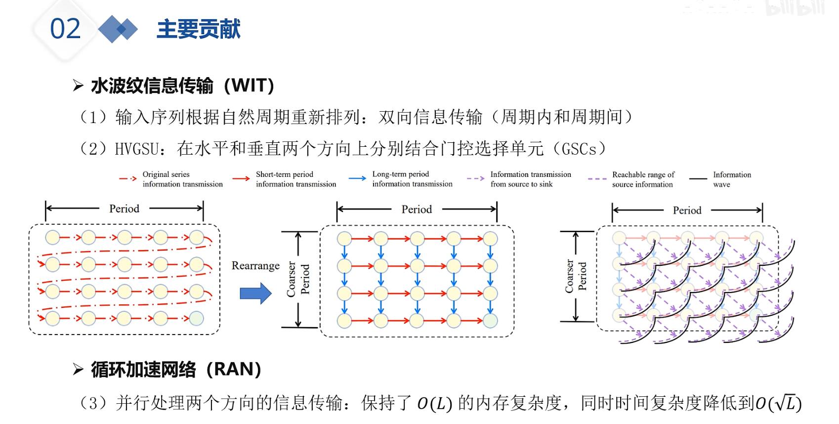
贡献：

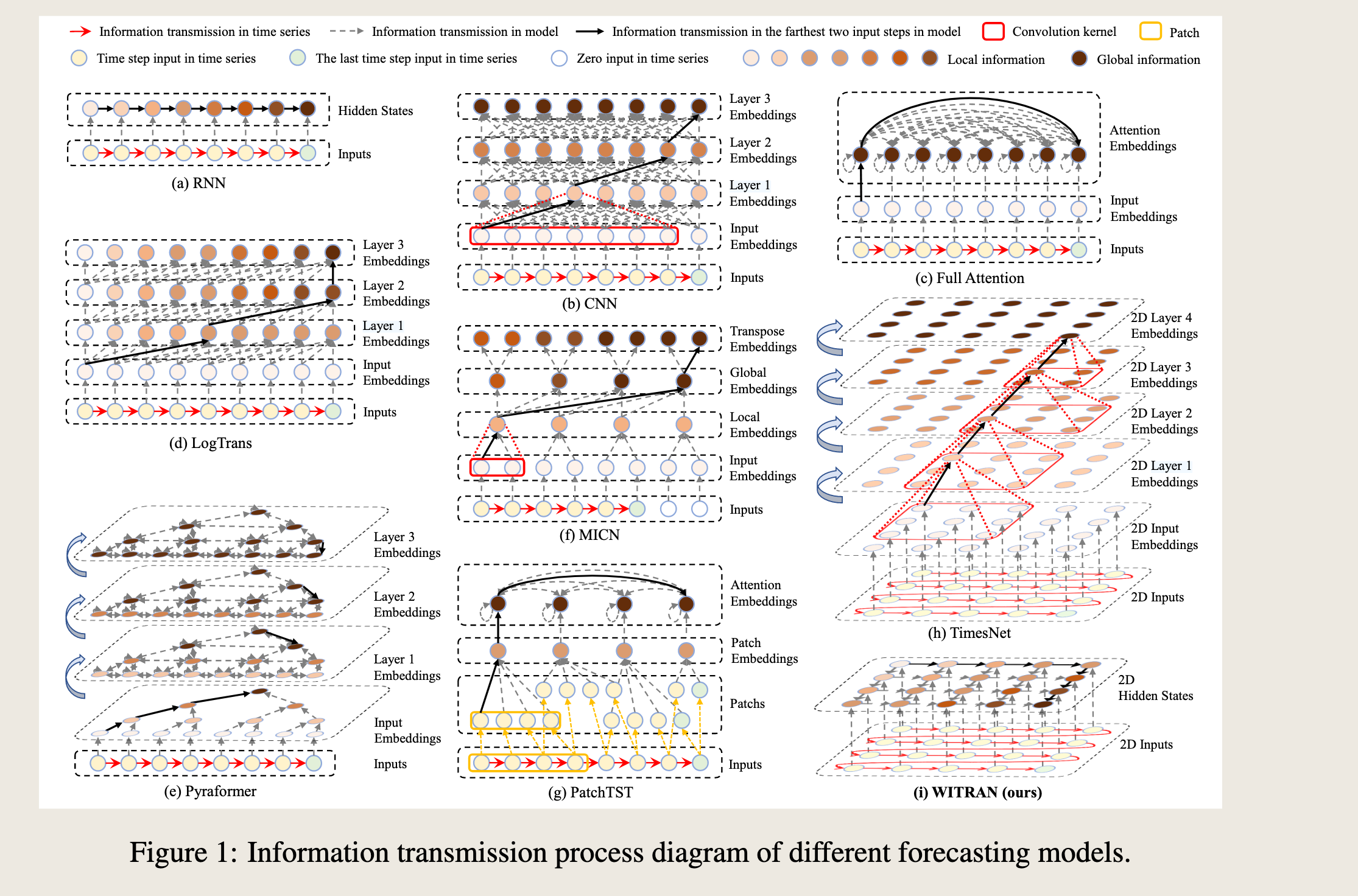
We propose a Water-wave Information Transmission and Recurrent Acceleration Network (WITRAN), which represents a novel paradigm in information transmission by enabling bi-granular flows. We provide a comprehensive comparison of WITRAN with previous methods in Figure 1 to highlight its uniqueness. Furthermore, in order to compare the differences between WITRAN and the model (a)-(h) in Figure 1 more clearly, we have prepared Table 1 to highlight the advantages of WITRAN.
我们提出了一种名为水波信息传输与递归加速网络（WITRAN）的新型信息传输范式，它通过实现双粒度信息流来代表信息传输的新方法。我们通过图1与之前的方法进行了全面的比较，以突出其独特性。此外，为了更清晰地比较WITRAN与图1中的模型（a）-（h）之间的差异，我们准备了表1来突出WITRAN的优势。
We propose a novel Horizontal Vertical Gated Selective Unit (HVGSU) which captures longand short-term periodic semantic information by using Gated Selective Cell (GSC) independently in both directions, preserving the characteristics of periodic semantic information. The fusion and selection in GSC can model the correlations of long- and short-term periodic semantic information. Furthermore, utilizing a recurrent structure with HVGSU facilitates the gradual capture of semantic information from local to global within a sequence.
我们提出了一种新型的水平垂直门控选择单元（HVGSU），该单元通过在两个方向上独立使用门控选择单元（GSC）来捕获长期和短期的周期性语义信息，同时保留周期性语义信息的特征。GSC中的融合和选择可以对长期和短期周期性语义信息的相关性进行建模。此外，利用包含HVGSU的递归结构有助于在序列中从局部到全局逐步捕获语义信息。
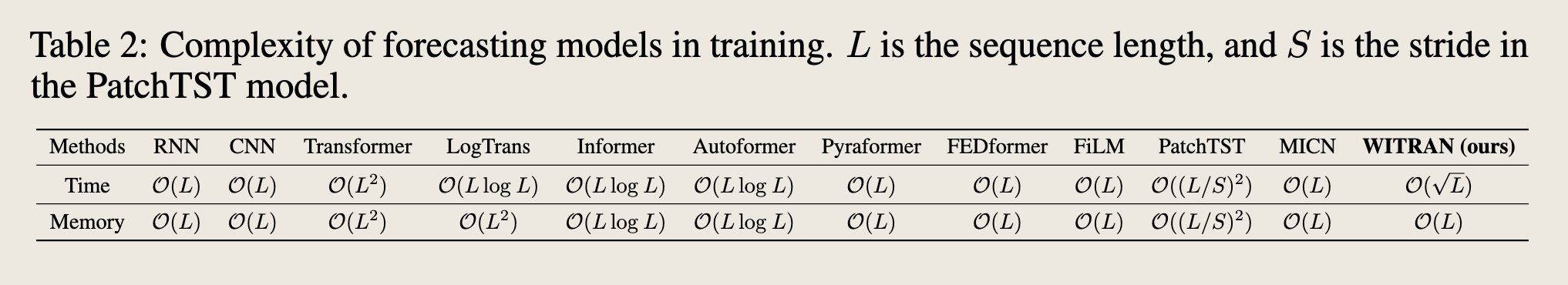
We present a Recurrent Acceleration Network (RAN) which is a generic acceleration framework that significantly reduces the time complexity to $\mathcal{O}(\sqrt{L})$ while maintaining the memory complexity of $\mathcal{O}(L)$ . We summarize the complexities of different methods in Table 2, demonstrating the superior efficiency of our method.
复杂度问题，时间复杂度&空间复杂度
循环加速框架

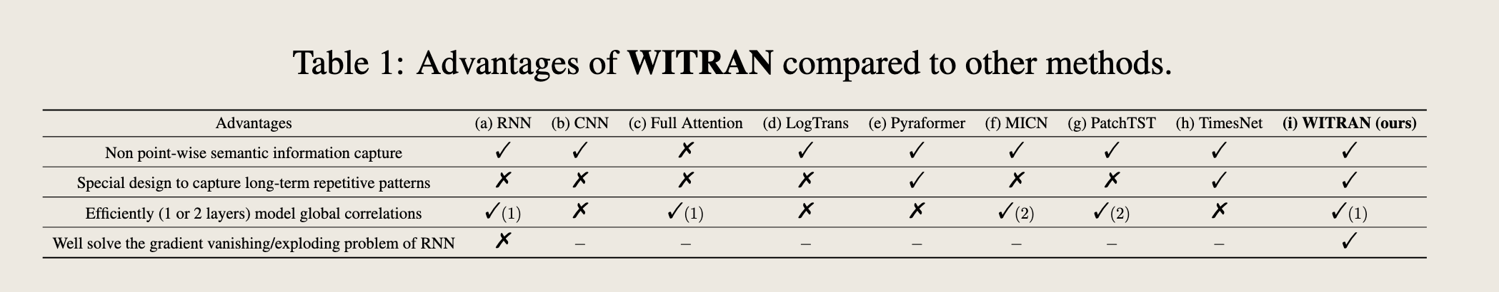
非逐点语义信息捕获
该能力指的是模型是否能够捕获非逐点的语义信息，即模型是否能够理解数据中的全局或整体模式，而不仅仅是单个点的信息。
RNN和CNN具有这种能力，而Full Attention、LogTrans、Pyraformer、MICN、PatchTST和TimesNet不具备。
WITRAN具备这种能力。
是否具备序列建模的能力
捕获长期周期性的特殊设计
该能力指的是模型是否具有专门设计来捕获时间序列中的长期重复模式。
LogTrans、Pyraformer、TimesNet和WITRAN具有这种能力，而RNN、CNN、Full Attention、MICN和PatchTST不具备。
WITRAN具备这种能力。
高效建模全局相关性
该能力指的是模型是否能够高效地（使用1或2层）建模全局相关性。
RNN、MICN和TimesNet具有这种能力，而CNN、Full Attention、LogTrans、Pyraformer和WITRAN不具备。
WITRAN具备这种能力。
解决 RNN 梯度爆炸和梯度消失问题
该能力指的是模型是否能够有效解决RNN中的梯度消失或爆炸问题。
只有WITRAN具备这种能力。

上表展示了不同模型的时间复杂度和空间复杂度
其中水波纹信息传输循环加速网络内存占用也是 $\mathcal{O}(L)$ ，但是时间复杂度优势显著 $\mathcal{O}(\sqrt{L})$
尤其对比 former 系的，Informer、Autoformer 通过稀疏自注意力机制将时间复杂度和内存复杂度降低到了 $\mathcal{O}(L\log {L})$
红色箭头表示原始序列的信息传输
红色虚线箭头表示短期周期信息传输
蓝色箭头表示长期周期信息传输
蓝色虚线箭头表示从源到汇的信息传输
虚线表示源信息的可达范围
实线表示信息波

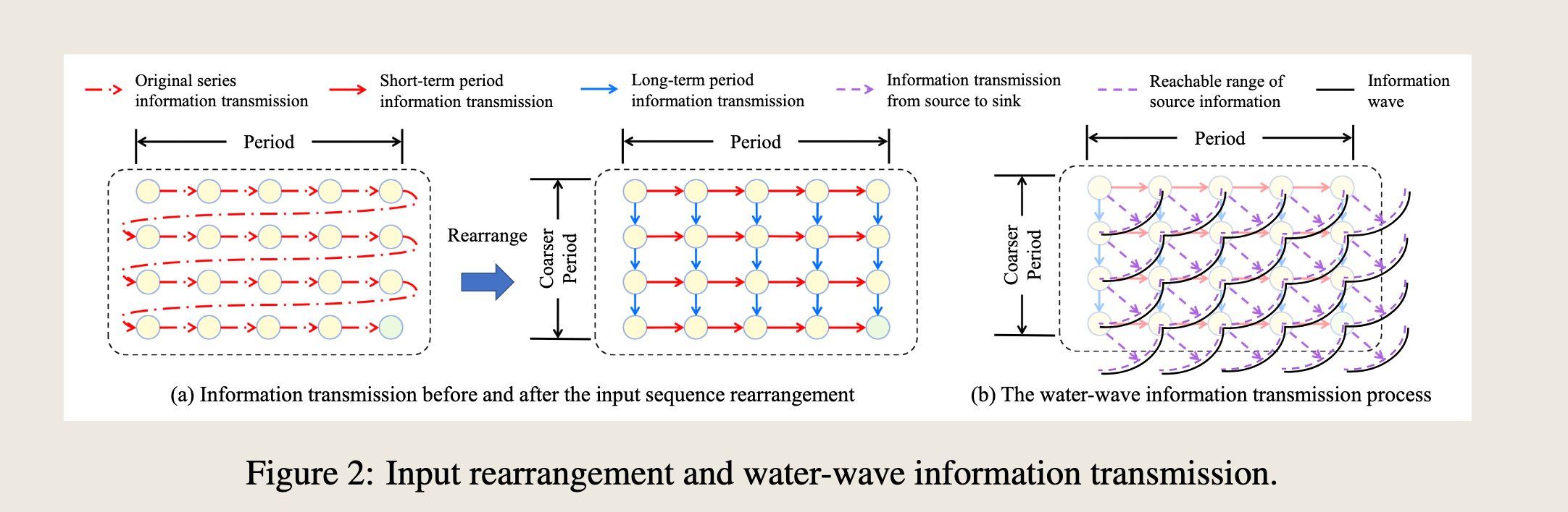
图 2 描述了时间序列数据的输入重排和水波信息传输过程。该图分为两个部分：

(a) 输入序列重排前后的信息传输

左侧图：展示了原始序列的信息传输。图中用红色箭头表示原始序列的信息传输，用红色虚线箭头表示短期周期信息传输。
右侧图：展示了输入序列重排后的信息传输。图中用蓝色箭头表示长期周期信息传输，用蓝色虚线箭头表示从源到汇的信息传输。
重排：通过重排输入序列，可以更有效地捕获长期信息，从而改善信息传输。

(b) 水波信息传输过程

图示：展示了水波信息传输的模拟过程。图中用实线表示信息波，用虚线表示源信息的可达范围。
过程：信息波从源点开始传播，随着时间的推移，信息波逐渐扩散并覆盖更广的范围。这种模拟有助于理解信息在时间序列中的传播和扩散过程。

图 2 说明了

输入重排可以改善信息传输，特别是长期信息的捕获；
水波信息传输模型提供了一种直观的方式来理解信息在时间序列中的传播和扩散

3 The WITRAN Model¶

The time series forecasting task involves predicting future values $Y \in \mathbb{R}^{P \times c_{\text{out}}}$ for $P$ time steps based on the historical input sequences $X = \{x_1, x_2, \ldots, x_H\} \in \mathbb{R}^{H \times c_{\text{in}}}$ of $H$ time steps, where $c_{\text{in}}$ and $c_{\text{out}}$ represent the number of input and output features respectively.

时间序列预测任务涉及基于历史输入序列 $X = \{x_1, x_2, \ldots, x_H\} \in \mathbb{R}^{H \times c_{\text{in}}}$ 预测未来 $P$ 个时间步长内的未来值 $Y \in \mathbb{R}^{P \times c_{\text{out}}}$，其中 $c_{\text{in}}$ 和 $c_{\text{out}}$ 分别表示输入和输出特征的数量。

In order to integrate enough historical information for analysis, it is necessary for $H$ to have a sufficient size [Liu et al., 2021, Zeng et al., 2023]. Furthermore, capturing semantic information from the historical input is crucial for accurate forecasting, which includes modeling global and local correlations, as well as discovering long- and short-term repetitive patterns.

为了整合足够的历史信息进行分析，$H$ 必须具有足够的大小 [Liu et al., 2021, Zeng et al., 2023]。此外，从历史输入中捕获语义信息对于准确预测至关重要，这包括建模全局和局部相关性以及发现长期和短期的重复模式。

However, how to address them simultaneously is a major challenge. With these in mind, we propose WITRAN, a novel information transmission framework akin to the propagation of water waves. WITRAN captures both long- and short-term periodic semantic information, as well as global-local semantic information simultaneously during information transmission. Moreover, WITRAN reduces time complexity while maintaining linear memory complexity. The overall structure of WITRAN is depicted in Figure 3.

然而，如何同时解决这些问题是一个主要挑战。基于这些考虑，我们提出了WITRAN，这是一种类似于水波传播的新型信息传输框架。WITRAN在信息传输过程中同时捕获长期和短期的周期性语义信息，以及全局-局部语义信息。此外，WITRAN在保持线性内存复杂度的同时降低了时间复杂度。WITRAN的整体结构如图3所示。

短期和长期的周星重复模式
内存复杂度：线性；时间复杂度 $\sqrt{L}$

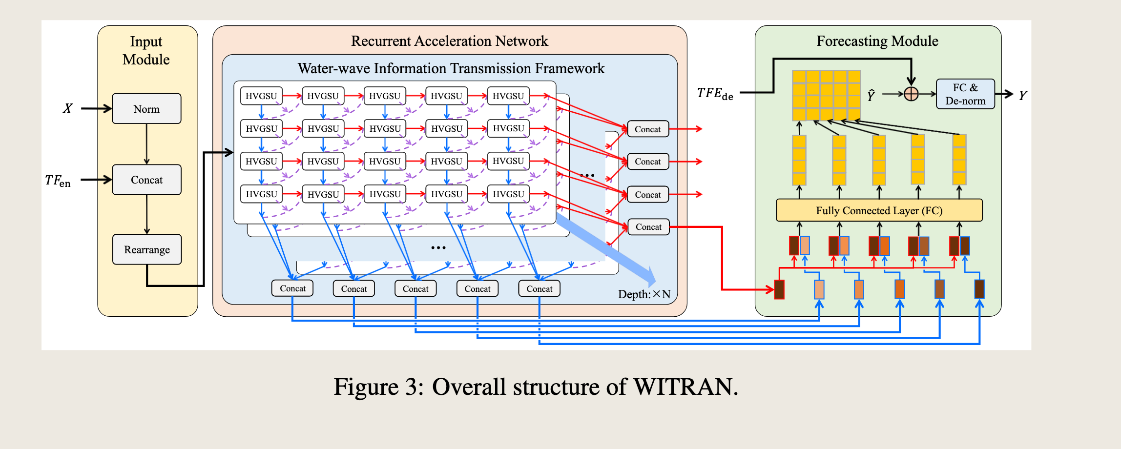
3.1 Input Module¶

To facilitate the analysis of long- and short-term repetitive patterns, inspired by TimesNet [Wu et al., 2023], we first rearrange the sequence from 1D to 2D based on its natural period, as illustrated by Figure 2(a).

为了便于分析长期和短期的重复模式，受TimesNet [Wu et al., 2023] 的启发，我们首先根据其自然周期将序列从一维重新排列为二维，如图2(a)所示。

Importantly, our approach involves analyzing the natural period of time series and setting appropriate hyperparameters to determine the input rearrangement, rather than using Fast Fourier Transform (FFT) to learn multiple adaptive periods of inputs in TimesNet.

重要的是，我们的方法涉及分析时间序列的自然周期，并设置适当的超参数来确定输入的重新排列，而不是使用快速傅里叶变换（FFT）来学习TimesNet中输入的多个自适应周期。

Consequently, our method is much simpler. Additionally, in order to minimize the distribution shift in datasets, we draw inspiration from NLinear [Zeng et al., 2023] and employ an adaptive learning approach to determine whether to perform simple normalization.

因此，我们的方法简单得多。此外，为了最小化数据集中的分布偏移，我们从NLinear [Zeng et al., 2023] 中汲取灵感，并采用自适应学习方法来决定是否执行简单的归一化。

The input module can be described as follows:

※ 输入模块可以描述如下： $$ X_{1D} = \begin{cases} X & , \text{norm} = 0 \ X - x_H & , \text{norm} = 1 \end{cases} $$

\[ X_{2D} = \text{Rearrange}([X_{1D}, TF_{en}]), \]

符号说明

$X_{1D} \in \mathbb{R}^{H \times c_{\text{in}}}$ 表示原始输入序列$x_H \in \mathbb{R}^{c_{\text{in}}}$ 表示原始序列最后一个时间步的输入
$TF_{en} \in \mathbb{R}^{H \times c_{\text{time}}}$ 表示原始输入序列的时间上下文特征（例如，HourOfDay、DayOfWeek、DayOfMonth 和 DayOfYear），其中 $c_{\text{time}}$ 是时间特征的维度。
$X_{2D} \in \mathbb{R}^{H \times C \times (c_{\text{in}} + c_{\text{time}})}$ 表示重新排列后的输入
其中 $R$ 表示水平行的总数
$C$ 表示垂直列
$\text{norm}$ 是不同任务的自适应参数
$[\cdot]$ 表示连接操作
$\text{Rearrange}$ 表示重新排列操作，参见图2(a)。

here, $X_{1D} \in \mathbb{R}^{H \times c_{\text{in}}}$ represents the original input sequences, $x_H \in \mathbb{R}^{c_{\text{in}}}$ represents the input at the last time step of the original sequence, $TF_{en} \in \mathbb{R}^{H \times c_{\text{time}}}$ represents the temporal contextual features of original input sequence (e.g., HourOfDay, DayOfWeek, DayOfMonth and DayOfYear), where $c_{\text{time}}$ is the dimension of time features. $X_{2D} \in \mathbb{R}^{H \times C \times (c_{\text{in}} + c_{\text{time}})}$ represents the inputs after rearrangement, where $R$ denotes the total number of horizontal rows and $C$ denotes the vertical columns. $\text{norm}$ is an adaptive parameter for different tasks. $[\cdot]$ represents the concat operation and $\text{Rearrange}$ represents the rearrange operation, with reference to Figure 2(a).

3.2 Horizontal Vertical Gated Selective Unit¶

To capture long- and short-term periodic semantic information and reserve their characteristics, we propose a novel Horizontal Vertical Gated Selective Unit (HVGSU) which consists of Gated Selective Cells (GSCs) in two directions.

为了捕获长期和短期的周期性语义信息并保留其特征，我们提出了一种新型的水平垂直门控选择单元（HVGSU），它由两个方向上的门控选择单元（GSCs）组成。

To capture the correlation at each time step between periodic semantic information of both directions, we design the specific operations in GSC.

为了捕获两个方向上周期性语义信息在每个时间步的关联，我们在GSC中设计了特定的操作。

Furthermore, HVGSU is capable of capturing both global and local information via a recurrent structure. In this subsection, we will provide a detailed introduction to them.

此外，HVGSU能够通过递归结构捕获全局和局部信息。在本小节中，我们将详细介绍它们。

HVGSU As depicted in Figure 3, the process of HVGSU via a recurrent structure is:

HVGSU 如图3所示，通过递归结构的HVGSU过程是： $$ H_{\text{hor}}, H_{\text{ver}}, \text{Out} = \text{HVGSU}(X_{2D}), $$ where $H_{\text{hor}} \in \mathbb{R}^{L \times R \times d_{\text{model}}}$ and $H_{\text{ver}} \in \mathbb{R}^{L \times C \times d_{\text{model}}}$ represent the horizontal and the vertical output hidden state of HVGSU separately. $L$ is the depth of the model, and $\text{Out} \in \mathbb{R}^{R \times C \times d_{\text{model}}}$ denotes the output information of the last layer.

其中 $H_{\text{hor}} \in \mathbb{R}^{L \times R \times d_{\text{model}}}$ $H_{\text{ver}} \in \mathbb{R}^{L \times C \times d_{\text{model}}}$ 分别表示HVGSU的水平和垂直输出隐藏状态。
$L$ 是模型的深度
$\text{Out} \in \mathbb{R}^{R \times C \times d_{\text{model}}}$ 表示最后一层的输出信息。

In greater detail, the cellular structure of HVGSU is shown in Figure 4(b), which consists of GSCs in two directions to capture the periodic semantic information of long- and short-term. The cell operations for row $r$ ($1 \leq r \leq R$) and column $c$ ($1 \leq c \leq C$) in layer $l$ ($1 \leq l \leq L$) can be formalized as:

更详细地说，HVGSU的细胞结构如图4(b)所示，它由两个方向上的GSC组成，以捕获长期和短期的周期性语义信息。对于层$l$（$1 \leq l \leq L$）中的行$r$（$1 \leq r \leq R$）和列$c$（$1 \leq c \leq C$）的单元操作可以形式化为： $$ h_{r,c,l}^{\text{hor}} = \text{GSC}{\text{hor}}(\text{input}_r, c, l, h) $$}^{\text{hor}}, h_{r-1,c,l}^{\text{ver}

\[ h_{r,c,l}^{\text{ver}} = \text{GSC}_{\text{ver}}(\text{input}_r, c, l, h_{r-1,c,l}^{\text{ver}}, h_{r,c-1,l}^{\text{hor}}) \]

\[ o_{r,c,l} = [h_{r,c,l}^{\text{hor}}, h_{r,c,l}^{\text{ver}}] \]

这里，$\text{input}_r, c, l \in \mathbb{R}^{d_{\text{in}}}$。
当$l = 1$时，$\text{input}_r, c, l = x_r, c \in \mathbb{R}^{c_{\text{in}} + c_{\text{time}}}$表示第一层的输入
当$l > 1$时，$\text{input}_r, c, l = o_r, c, l-1 \in \mathbb{R}^{2 \times d_{\text{model}}}$表示后续层的输入
$h_{r,c-1,l}^{\text{hor}}$ 和 $h_{r-1,c,l}^{\text{ver}} \in \mathbb{R}^{d_{\text{model}}}$ 分别表示当前单元的水平和垂直隐藏状态输入。
注意，当$r = 1$时，$h_{r-1,c,l}^{\text{ver}}$被替换为相同大小的全零张量
当$c = 1$时，$h_{r,c-1,l}^{\text{hor}}$也是如此
$[\cdot]$表示连接操作
$o_{r,c,l} \in \mathbb{R}^{2 \times d_{\text{model}}}$表示当前单元的输出。

here, $\text{input}_r, c, l \in \mathbb{R}^{d_{\text{in}}}$. When $l = 1$, $\text{input}_r, c, l = x_r, c \in \mathbb{R}^{c_{\text{in}} + c_{\text{time}}}$ represents the input for the first layer, and when $l > 1$, $\text{input}_r, c, l = o_r, c, l-1 \in \mathbb{R}^{2 \times d_{\text{model}}}$ represents the input for subsequent layers. $h_{r,c-1,l}^{\text{hor}}$ and $h_{r-1,c,l}^{\text{ver}} \in \mathbb{R}^{d_{\text{model}}}$ represent the horizontal and vertical hidden state inputs of the current cell. Note that when $r = 1$, $h_{r-1,c,l}^{\text{ver}}$ is replaced by an all-zero tensor of the same size, and the same is true for $h_{r,c-1,l}^{\text{hor}}$ when $c = 1$. $[\cdot]$ represents the concat operation and $o_{r,c,l} \in \mathbb{R}^{2 \times d_{\text{model}}}$ represents the output of the current cell.

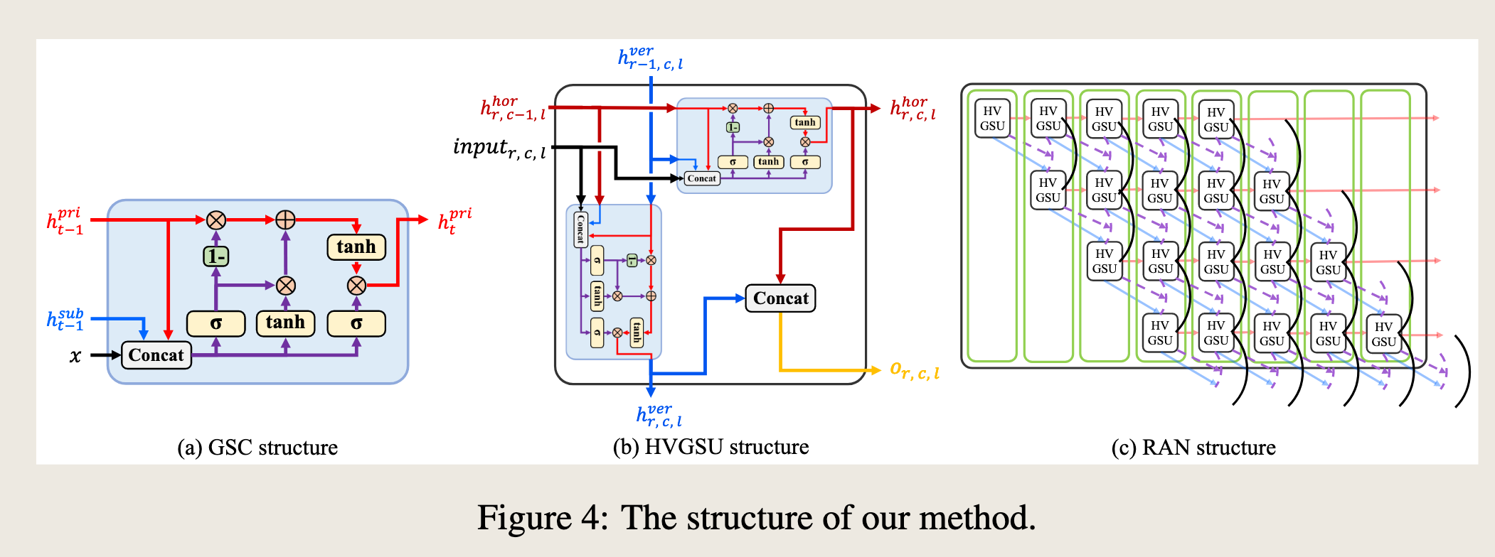
GSC Inspired by the two popular RNN-based models, LSTM [Hochreiter and Schmidhuber, 1997] and GRU [Chung et al., 2014] (for more details, see Appendix A), we propose a Gated Selective Cell (GSC) to fuse and select information.

门控选择单元（GSC） 受两个流行的基于循环神经网络（RNN）的模型——长短期记忆网络（LSTM）[Hochreiter 和 Schmidhuber, 1997] 和门控循环单元（GRU）[Chung 等, 2014]（更多细节见附录A）的启发，我们提出了一种门控选择单元（GSC）来融合和选择信息。

Its structure is shown in Figure 4(a), which comprises two gates: the selection gate, and the output gate. The fused information consists of input and principal-subordinate hidden states, and the selection gate determines the retention of the original principal information and the addition of the fused information. Finally, the output gate determines the final output information of the cell.

其结构如图4(a)所示，包括两个门：选择门和输出门。融合的信息由输入和主从隐藏状态组成，选择门决定了原始主信息的保留和融合信息的添加。最后，输出门决定了单元的最终输出信息。

The different colored arrows in Figure 4(a) represent different semantic information transfer processes. The black arrow represents the input, the red arrows represent the process of transmitting principal hidden state information, the blue arrow represents the subordinate hidden state, and the purple arrows represent the process by which fused information of principal-subordinate hidden states is transmitted. The formulations are given as follows:

图4(a)中不同颜色的箭头代表不同的语义信息传递过程。黑色箭头代表输入，红色箭头代表主隐藏状态信息传递的过程，蓝色箭头代表从隐藏状态，紫色箭头代表主从隐藏状态融合信息传递的过程。公式如下所示：

\[ S_t = \sigma(W_s[h_{t-1}^{\text{pri}}, h_{t-1}^{\text{sub}}, x] + b_s) \]

\[ O_t = \sigma(W_o[h_{t-1}^{\text{pri}}, h_{t-1}^{\text{sub}}, x] + b_o) \]

\[ h_f = \tanh(W_f[h_{t-1}^{\text{pri}}, h_{t-1}^{\text{sub}}, x] + b_f) \]

\[ \widetilde{h_{t-1}^{\text{pri}}} = (1 - S_t) \odot h_{t-1}^{\text{pri}} + S_t \odot h_f \]

\[ h_t^{\text{pri}} = \tanh(\widetilde{h_{t-1}^{\text{pri}}}) \odot O_t, \]

where $h_{t-1}^{\text{pri}}$ and $h_{t-1}^{\text{sub}} \in \mathbb{R}^{d_{\text{model}}}$ represent the input principal and subordinate hidden state, $x \in \mathbb{R}^{d_{\text{in}}}$ represents the input.

其中 $h_{t-1}^{\text{pri}}$ 和 $h_{t-1}^{\text{sub}} \in \mathbb{R}^{d_{\text{model}}}$ 分别表示输入的主隐藏状态和从隐藏状态，$x \in \mathbb{R}^{d_{\text{in}}}$ 表示输入。

$W_* \in \mathbb{R}^{d_{\text{model}} \times (2d_{\text{model}} + d_{\text{in}})}$ are weight matrices and $b_* \in \mathbb{R}^{d_{\text{model}}}$ are bias vectors.

$W_* \in \mathbb{R}^{d_{\text{model}} \times (2d_{\text{model}} + d_{\text{in}})}$ 是权重矩阵，$b_* \in \mathbb{R}^{d_{\text{model}}}$ 是偏置向量。

$S_t$ and $O_t$ denote the selection gate and the output gate, $\odot$ denotes an element-wise product, $\sigma(\cdot)$ and $\tanh(\cdot)$ denote the sigmoid and tanh activation function.

$S_t$ 和 $O_t$ 分别表示选择门和输出门，$\odot$ 表示元素级乘积，$\sigma(\cdot)$ 和 $\tanh(\cdot)$ 分别表示sigmoid和tanh激活函数。

$h_f$ and $\widetilde{h_{t-1}^{\text{pri}}} \in \mathbb{R}^{d_{\text{model}}}$ represent the intermediate variables of the calculation. $h_t^{\text{pri}}$ represents the output hidden state.

$h_f$ 和 $\widetilde{h_{t-1}^{\text{pri}}} \in \mathbb{R}^{d_{\text{model}}}$ 表示计算过程中的中间变量。$h_t^{\text{pri}}$ 表示输出隐藏状态。

3.3 Recurrent Acceleration Network¶

In traditional recurrent structure, for two adjacent time steps in series, the latter one always waits for the former one until the information computation of the former one is completed. When the sequence becomes longer, this becomes slower.

在传统的递归结构中，对于序列中的两个相邻时间步，后者总是要等待前者完成信息计算。当序列变长时，这会导致速度变慢。

Fortunately, in the WIT framework we designed, some of the time step information can be computed in parallel.

幸运的是，在我们设计的水波信息传输（WIT）框架中，部分时间步信息可以并行计算。

As shown in Figure 2(b), after a point is calculated, the right point in its horizontal direction and the point below it in its vertical direction can start calculation without waiting for each other.

如图2(b)所示，在计算出一个点之后，其水平方向上的右侧点和垂直方向上的下方点可以开始计算而无需等待彼此。

Therefore, we propose the Recurrent Acceleration Network (RAN) as our accelerated framework, which enables parallel computation of data points without waiting for each other, greatly improving the efficiency of information transmission in HVGSU.

因此，我们提出了递归加速网络（RAN）作为我们的加速框架，它能够在不等待彼此的情况下并行计算数据点，从而大大提高了HVGSU中信息传输的效率。

We place parallelizable points in a slice, and the updated information transfer process is shown in Figure 4(c). Each green box in Figure 4(c) represents a slice, and the number of green boxes is the number of times we need to recursively compute.

我们将可并行化的点放置在一个切片中，更新的信息传输过程如图4(c)所示。图4(c)中的每个绿色框代表一个切片，绿色框的数量是我们递归计算所需的次数。

The meanings of the remaining markers are the same as those in Figure 2. Under the RAN framework, the recurrent length has changed from the sequence length $L = R \times C$ to $R + C - 1$, while the complexity of $R$ and $C$ is $O(\sqrt{L})$.

剩余标记的含义与图2中的相同。在RAN框架下，递归长度从序列长度 $L = R \times C$ 变为 $R + C - 1$，而 $R$ 和 $C$ 的复杂度为 $O(\sqrt{L})$。

Thus, we have reduced the time complexity to $O(\sqrt{L})$ via the RAN framework. It should be noted that although we parallelly compute some data points, which may increase some memory, the complexity of parallel computation, $O(\sqrt{L})$, is far less than the complexity of saving the output variables, $O(L)$, because we need to save the output information of each point in the sequence. Implementation source code for RAN is given in Appendix D.

因此，我们通过RAN框架将时间复杂度降低到 $O(\sqrt{L})$。需要注意的是，尽管我们并行计算了一些数据点，这可能会增加一些内存，但并行计算的复杂度 $O(\sqrt{L})$ 远小于保存输出变量的复杂度 $O(L)$，因为我们需要保存序列中每个点的输出信息。RAN的实现源代码在附录D中给出。

3.4 Forecasting Module¶

In the forecasting module, we address the issue of error accumulation in the auto-regressive structure by drawing inspiration from Informer [Zhou et al., 2021] and Pyraformer [Liu et al., 2021], combining both horizontal and vertical hidden states, and then making predictions through a fully connected layer, as illustrated in Figure 3.

在预测模块中，我们借鉴了Informer [Zhou et al., 2021] 和 Pyraformer [Liu et al., 2021] 的方法，通过结合水平和垂直隐藏状态来解决自回归结构中的误差累积问题，然后通过一个全连接层进行预测，如图3所示。

We utilize the last row of the horizontal hidden states as it contains sufficient global and latest shortterm semantic information from the historical sequence.

我们利用水平隐藏状态的最后一行，因为它包含了来自历史序列的充足全局和最新短期语义信息。

In contrast, all columns of the vertical hidden states, which capture different long-term semantic information, are all preserved.

相比之下，垂直隐藏状态的所有列都捕获了不同的长期语义信息，因此都被保留。

The combined operation not only maximizes the retention of the various semantic information needed for predicting the points, but also avoids excessive redundancy in order to obtain accurate predictions. This module can be formalized as follows:

这种组合操作不仅最大化了保留预测点所需的各种语义信息，还避免了过度冗余，以获得准确的预测。该模块可以公式化表示如下： $$ H_{\text{hor}}^{\text{rep}} = \text{Repeat}(h_{\text{hor}}) $$

\[ H_{h-v} = \text{Reshape}([H_{\text{hor}}^{\text{rep}}, H_{\text{ver}}]) \]

\[ \hat{Y} = \text{FC1}(H_{h-v}) \]

\[ Y = \text{FC2}(\text{Reshape}(\hat{Y}) + TFE_{\text{de}}) \]

where $TFE_{\text{de}} \in \mathbb{R}^{P \times C \times d_{\text{model}}}$ represents time features encoding of the forecasting points separately.
$TFE_{\text{de}} \in \mathbb{R}^{P \times C \times d_{\text{model}}}$ 表示分别对预测点进行时间特征编码。
$h_{\text{hor}} \in \mathbb{R}^{L \times 1 \times d_{\text{model}}}$ represents the last row hidden state in $H_{\text{hor}}$.
$h_{\text{hor}} \in \mathbb{R}^{L \times 1 \times d_{\text{model}}}$ 表示 $H_{\text{hor}}$ 中的最后一行隐藏状态。
Repeat(·) is for repeat operation and Reshape(·) is for reshape operation. FC1 and FC2 represent two fully connected layers respectively.
Repeat(·) 是重复操作，Reshape(·) 是重塑操作。FC1 和 FC2 分别表示两个全连接层。
$\hat{Y} \in \mathbb{R}^{C \times (R_{\text{de}} \times d_{\text{model}})}$ represents the intermediate variables of the calculation and $R_{\text{de}} \times C = P$.
$\hat{Y} \in \mathbb{R}^{C \times (R_{\text{de}} \times d_{\text{model}})}$ 表示计算的中间变量，且 $R_{\text{de}} \times C = P$。
$Y$ represents the output of this module, and it is worth noting that we need to utilize the adaptive parameter $norm$ for denormalization, when $norm = 1$, $Y = Y + x_H$.
$Y$ 表示该模块的输出，值得注意的是，我们需要利用自适应参数 $norm$ 进行反归一化，当 $norm = 1$ 时，$Y = Y + x_H$。

论文研读¶

参看链接：论文研读之长程时序预测：水波纹信息传输WIT和循环加速网络RAN

问题描述：

精准的远程和超远程时序预测：使用更长的历史序列作为输入
捕获语义信息
考虑建模效率

add_circle2025-04-13 13:02:21update2025-04-14 20:21:33