2022、LTSF-Linear¶

约 20999 个字 20 张图片预计阅读时间 105 分钟

原文：Are Transformers Effective for Time Series Forecasting?

源码：https://github.com/cure-lab/LTSF-Linear

Abstract¶

Recently, there has been a surge of Transformer-based solutions for the long-term time series forecasting (LTSF) task. Despite the growing performance over the past few years, we question the validity of this line of research in this work.

近期，基于Transformer的解决方案在长期时间序列预测（LTSF）任务中呈现出迅猛发展的态势。尽管过去几年其性能不断提升，但我们在本研究中对该研究方向的有效性提出了质疑。

Specifically, Transformers is arguably the most successful solution to extract the semantic correlations among the elements in a long sequence. However, in time series modeling, we are to extract the temporal relations in an ordered set of continuous points.

具体而言，Transformer无疑是提取长序列中元素之间语义关联最为成功的解决方案。然而，在时间序列建模中，我们的目标是从连续点的有序集合中提取时间关系。

While employing positional encoding and using tokens to embed sub-series in Transformers facilitate preserving some ordering information, the nature of the permutation-invariant self-attention mechanism inevitably results in temporal information loss.

虽然在Transformer中使用位置编码以及利用标记嵌入子序列有助于保留部分顺序信息，但排列不变的自注意力机制的固有特性不可避免地会导致时间信息的丢失。

To validate our claim, we introduce a set of embarrassingly simple one-layer linear models named LTSF-Linear for comparison. Experimental results on nine real-life datasets show that LTSF-Linear surprisingly outperforms existing sophisticated Transformer-based LTSF models in all cases, and often by a large margin.

Moreover, we conduct comprehensive empirical studies to explore the impacts of various design elements of LTSF models on their temporal relation extraction capability. We hope this surprising finding opens up new research directions for the LTSF task. We also advocate revisiting the validity of Transformer-based solutions for other time series analysis tasks (e.g., anomaly detection) in the future. Code is available at: https://github.com/cure-lab/LTSFLinear.

为了验证我们的观点，我们引入了一组极其简单的单层线性模型，命名为 LTSF-Linear，用于对比。在九个真实数据集上的实验结果显示，LTSF-Linear 意外地在所有情况下均优于现有的复杂基于 Transformer 的 LTSF 模型，且通常优势显著。

此外，我们还进行了全面的实证研究，以探索 LTSF 模型的各种设计元素对其时间关系提取能力的影响。我们希望这一令人意外的发现能够为 LTSF 任务开辟新的研究方向。我们还倡导在未来重新审视基于 Transformer 的解决方案在其他时间序列分析任务（例如异常检测）中的有效性。代码可在以下链接获取：https://github.com/cure-lab/LTSFLinear。

1. Introduction¶

Time series are ubiquitous in today’s data-driven world. Given historical data, time series forecasting (TSF) is a long-standing task that has a wide range of applications, including but not limited to traffic flow estimation, energy management, and financial investment. Over the past several decades, TSF solutions have undergone a progression from traditional statistical methods (e.g., ARIMA [1]) and machine learning techniques (e.g., GBRT [11]) to deep learning-based solutions, e.g., Recurrent Neural Networks [15] and Temporal Convolutional Networks [3, 17].

在当今数据驱动的世界中，时间序列无处不在。基于历史数据，时间序列预测（TSF）是一项由来已久的任务，其应用范围极为广泛，包括但不限于交通流量估计、能源管理和金融投资等领域。在过去几十年间，时间序列预测的解决方案经历了从传统的统计方法（例如ARIMA）和机器学习技术（例如GBRT）到基于深度学习的解决方案（例如循环神经网络和时间卷积网络）的发展演变。

Transformer [26] is arguably the most successful sequence modeling architecture, demonstrating unparalleled performances in various applications, such as natural language processing (NLP) [7], speech recognition [8], and computer vision [19, 29]. Recently, there has also been a surge of Transformer-based solutions for time series analysis, as surveyed in [27]. Most notable models, which focus on the less explored and challenging long-term time series forecasting (LTSF) problem, include LogTrans [16] (NeurIPS 2019), Informer [30] (AAAI 2021 Best paper), Autoformer [28] (NeurIPS 2021), Pyraformer [18] (ICLR 2022 Oral), Triformer [5] (IJCAI 2022) and the recent FEDformer [31] (ICML 2022).

Transformer无疑是序列建模领域最为成功的架构，在诸多应用中展现出了无与伦比的性能，例如自然语言处理（NLP）、语音识别以及计算机视觉等。近期，基于Transformer的时间序列分析解决方案也呈现出迅猛发展的态势，相关研究综述可见于文献[27]。其中，专注于长期时间序列预测（LTSF）这一尚未充分探索且极具挑战性的问题的最具代表性的模型包括LogTrans[16]（NeurIPS 2019）、Informer[30]（AAAI 2021最佳论文）、Autoformer[28]（NeurIPS 2021）、Pyraformer[18]（ICLR 2022口头报告）、Triformer[5]（IJCAI 2022）以及最近的FEDformer[31]（ICML 2022）。

The main working power of Transformers is from its multi-head self-attention mechanism, which has a remarkable capability of extracting semantic correlations among elements in a long sequence (e.g., words in texts or 2D patches in images). However, self-attention is permutationinvariant and “anti-order” to some extent. While using various types of positional encoding techniques can preserve some ordering information, it is still inevitable to have temporal information loss after applying self-attention on top of them.

Transformer的主要工作原理源于其多头自注意力机制，该机制在提取长序列中元素之间的语义关联（例如文本中的词语或图像中的二维块）方面具有显著的能力。然而，自注意力机制是排列不变的，并且在某种程度上是“反序”的。尽管使用各种类型的位置编码技术可以保留一些顺序信息，但在应用自注意力之后，仍然不可避免地会导致时间信息的丢失。

This is usually not a serious concern for semanticrich applications such as NLP, e.g., the semantic meaning of a sentence is largely preserved even if we reorder some words in it. However, when analyzing time series data, there is usually a lack of semantics in the numerical data itself, and we are mainly interested in modeling the temporal changes among a continuous set of points. That is, the order itself plays the most crucial role. Consequently, we pose the following intriguing question: Are Transformers really effective for long-term time series forecasting?

对于语义丰富的应用（如自然语言处理），这通常不是严重的问题，例如，即使我们重新排列句子中的一些词语，句子的语义意义仍然得以大部分保留。然而，在分析时间序列数据时，数值数据本身通常缺乏语义，而我们主要关注的是建模连续点集之间的时间变化。也就是说，顺序本身起着最关键的作用。因此，我们提出了以下引人入胜的问题：Transformer是否真的适用于长期时间序列预测？

Moreover, while existing Transformer-based LTSF solutions have demonstrated considerable prediction accuracy improvements over traditional methods, in their experiments, all the compared (non-Transformer) baselines perform autoregressive or iterated multi-step (IMS) forecasting [1, 2, 22, 24], which are known to suffer from significant error accumulation effects for the LTSF problem. Therefore, in this work, we challenge Transformer-based LTSF solutions with direct multi-step (DMS) forecasting strategies to validate their real performance.

此外，尽管现有的基于Transformer的长期时间序列预测（LTSF）解决方案已显示出相较于传统方法的显著预测精度提升，但在其实验中，所有被比较的（非Transformer）基线均采用自回归或迭代多步（IMS）预测策略。这些方法已知在LTSF问题中存在显著的误差累积效应。因此，在本工作中，我们采用直接多步（DMS）预测策略来挑战基于Transformer的LTSF解决方案，以验证其真实性能。

还是得多看文献，现在都是多步并行预测

Not all time series are predictable, let alone long-term forecasting (e.g., for chaotic systems).

We hypothesize that long-term forecasting is only feasible for those time series with a relatively clear trend and periodicity.

As linear models can already extract such information, we introduce a set of embarrassingly simple models named LTSF-Linear as a new baseline for comparison.

LTSF-Linear regresses historical time series with a one-layer linear model to forecast future time series directly.

并非所有时间序列都具备可预测性，长期预测更是如此（例如混沌系统）。我们推测，长期预测仅适用于那些趋势和周期性较为明显的时间序列。由于线性模型已经能够提取此类信息，我们引入了一组极为简单的模型，命名为 LTSF-Linear，作为新的比较基线。LTSF-Linear 通过单层线性模型对历史时间序列进行回归，直接预测未来的序列。

We conduct extensive experiments on nine widely-used benchmark datasets that cover various real-life applications: traffic, energy, economics, weather, and disease predictions.

Surprisingly, our results show that LTSF-Linear outperforms existing complex Transformerbased models in all cases, and often by a large margin (20% ∼ 50%).

Moreover, we find that, in contrast to the claims in existing Transformers, most of them fail to extract temporal relations from long sequences, i.e., the forecasting errors are not reduced (sometimes even increased) with the increase of look-back window sizes.

Finally, we conduct various ablation studies on existing Transformer-based TSF solutions to study the impact of various design elements in them.

我们在涵盖交通、能源、经济、天气和疾病预测等多种实际应用的九个广泛使用的基准数据集上进行了大量实验。令人意外的是，结果显示 LTSF-Linear 在所有情况下均优于现有的复杂基于 Transformer 的模型，且优势显著（20% 至 50%）。

此外，我们发现，与现有 Transformer 中的主张相反，大多数 Transformer 无法从长序列中提取时间关系，即随着回顾窗口大小的增加，预测误差并未降低（有时甚至增加）。最后，我们对现有的基于 Transformer 的时间序列预测（TSF）解决方案进行了各种消融研究，以探究其中各种设计元素的影响。

所以说，Transformer 的回望窗口边长误差会增加

contributions¶

To sum up, the contributions of this work include:

To the best of our knowledge, this is the first work to challenge the effectiveness of the booming Transformers for the long-term time series forecasting task.
据我们所知，这是首次对在长期时间序列预测任务中蓬勃发展的Transformer的有效性提出挑战。
To validate our claims, we introduce a set of embarrassingly simple one-layer linear models, named LTSF-Linear, and compare them with existing Transformer-based LTSF solutions on nine benchmarks. LTSF-Linear can be a new baseline for the LTSF problem.
为了验证我们的观点，我们引入了一组极其简单的单层线性模型，命名为LTSF-Linear，并在九个基准数据集上将其与现有的基于Transformer的LTSF解决方案进行比较。LTSF-Linear可以作为LTSF问题的一个新的基线模型。
We conduct comprehensive empirical studies on various aspects of existing Transformer-based solutions, including the capability of modeling long inputs, the sensitivity to time series order, the impact of positional encoding and sub-series embedding, and efficiency comparisons. Our findings would benefit future research in this area.
我们对现有基于Transformer的解决方案的各个方面进行了全面的实证研究，包括对长输入的建模能力、对时间序列顺序的敏感性、位置编码和子序列嵌入的影响以及效率比较等。我们的发现将有助于该领域未来的研究。

With the above, we conclude that ① the temporal modeling capabilities of Transformers for time series are exaggerated, at least for the existing LTSF benchmarks. At the same time, ② while LTSF-Linear achieves a better prediction accuracy compared to existing works, it merely serves as a simple baseline for future research on the challenging longterm TSF problem.

With our findings, we also advocate revisiting the validity of Transformer-based solutions for other time series analysis tasks in the future.

基于上述研究，我们得出结论：Transformer在时间序列建模方面的能力被高估了，至少对于现有的长期时间序列预测（LTSF）基准测试而言是这样。与此同时，尽管LTSF-Linear相较于现有研究实现了更高的预测精度，但它仅仅是一个简单的基线模型，用于未来对极具挑战性的长期时间序列预测（TSF）问题的研究。鉴于我们的发现，我们还倡导在未来重新审视基于Transformer的解决方案在其他时间序列分析任务中的有效性。

2. Preliminaries: TSF Problem Formulation¶

For time series containing C variates, given historical data $ \mathcal{X} = {X_1^t, ..., X_C^t}_{t=1}L $, wherein L is the look-back window size and $ X_i^t $ is the value of the i^th variate at the t^th time step. The time series forecasting task is to predict the values $ \hat{\mathcal{X}} = {\hat{X}_1^t, ..., \hat{X}_C^t}_{t=L+1} $ at the T future time steps.

When T > 1, iterated multi-step (IMS) forecasting learns a single-step forecaster and iteratively applies it to obtain multi-step predictions. Alternatively, direct multi-step (DMS) forecasting directly optimizes the multi-step forecasting objective at once.

对于包含 C 个变量的时间序列，给定历史数据 $ \mathcal{X} = {X_1^t, ..., X_C^t}_{t=1}L $，其中 L 是回溯窗口大小，$ X_i^t $ 是第 i 个变量在第 t 个时间步的值。时间序列预测任务是预测未来 T 个时间步的值 $ \hat{\mathcal{X}} = {\hat{X}_1^t, ..., \hat{X}_C^t}_{t=L+1} $。当 T > 1 时，迭代多步（IMS）预测学习一个单步预测器，并迭代地应用它来获得多步预测。或者，直接多步（DMS）预测直接一次性优化多步预测目标。

Compared to DMS forecasting results, IMS predictions have smaller variance thanks to the autoregressive estimation procedure, but they inevitably suffer from error accumulation effects.

Consequently, IMS forecasting is preferable when there is a highly-accurate single-step forecaster, and $T$ is relatively small.

In contrast, DMS forecasting generates more accurate predictions when it is hard to obtain an unbiased single-step forecasting model, or $T$ is large.

与直接多步（DMS）预测结果相比，迭代多步（IMS）预测由于自回归估计过程而具有较小的方差，但它们不可避免地会遭受误差累积效应的影响。因此，当存在高度精确的单步预测器，且 $T$ 相对较小时，IMS预测更为可取。相反，当难以获得无偏的单步预测模型，或者 $T$ 较大时，DMS预测能够生成更准确的预测。

这部分讨论了什么时候使用自回归预测，什么时候采用并行预测

那我的预测逻辑是有点问题

收获：并行多步预测；还有一个问题，是采用通道独立策略还是混合

3. Transformer-Based LTSF Solutions¶

Transformer-based models [26] have achieved unparalleled performances in many long-standing AI tasks in natural language processing and computer vision fields, thanks to the effectiveness of the multi-head self-attention mechanism.

This has also triggered lots of research interest in Transformer-based time series modeling techniques [20, 27].

In particular, a large amount of research works are dedicated to the LTSF task (e.g., [16, 18, 28, 30, 31]). Considering the ability to capture long-range dependencies with Transformer models, most of them focus on the less-explored long-term forecasting problem ($T \gg 1$) [1].

基于Transformer的模型[26]由于多头自注意力机制的有效性，在自然语言处理和计算机视觉领域的许多长期存在的AI任务中取得了无与伦比的性能。这也激发了对基于Transformer的时间序列建模技术[20, 27]的大量研究兴趣。特别是，大量的研究工作致力于长期时间序列预测（LTSF）任务（例如，[16, 18, 28, 30, 31]）。考虑到使用Transformer模型捕捉长距离依赖关系的能力，他们中的大多数都集中在探索较少的长期预测问题（$T \gg 1$）[1]。

所以长期预测问题，反而是 Transformer 出现以后开始的

When applying the vanilla Transformer model to the LTSF problem, it has some limitations, including the quadratic time/memory complexity with the original selfattention scheme and error accumulation caused by the autoregressive decoder design. Informer [30] addresses these issues and proposes a novel Transformer architecture with reduced complexity and a DMS forecasting strategy. Later, more Transformer variants introduce various time series features into their models for performance or efficiency improvements [18,28,31]. We summarize the design elements of existing Transformer-based LTSF solutions as follows (see Figure 1).

将经典的Transformer模型应用于长期时间序列预测（LTSF）问题时，存在一些限制，包括原始自注意力机制的二次时间和内存复杂度以及由自回归解码器设计引起的误差累积。Informer [30] 解决了这些问题，并提出了一种具有降低复杂度和直接多步（DMS）预测策略的新型Transformer架构。随后，更多的Transformer变体将各种时间序列特征引入他们的模型中，以提高性能或效率[18, 28, 31]。我们如下总结了现有基于Transformer的LTSF解决方案的设计元素（见图1）。

指出 Transformer 对于时序任务的问题：二次时间复杂度&空间复杂度

Informer，降低复杂度&直接多步预测（mark）

Time series decomposition: For data preprocessing, normalization with zero-mean is common in TSF. Besides, Autoformer [28] first applies seasonal-trend decomposition behind each neural block, which is a standard method in time series analysis to make raw data more predictable [6, 13]. Specifically, they use a moving average kernel on the input sequence to extract the trend-cyclical component of the time series. The difference between the original sequence and the trend component is regarded as the seasonal component. On top of the decomposition scheme of Autoformer, FEDformer [31] further proposes the mixture of experts’ strategies to mix the trend components extracted by moving average kernels with various kernel sizes.

时间序列分解：在数据预处理中，零均值归一化在时间序列预测（TSF）中很常见。此外，Autoformer[28]首次在每个神经块后面应用季节趋势分解，这是时间序列分析中使原始数据更可预测的标准方法[6, 13]。具体来说，他们使用移动平均核在输入序列上提取时间序列的趋势周期成分。原始序列与趋势成分之间的差值被视为季节成分。在Autoformer的分解方案基础上，FEDformer[31]进一步提出了专家混合策略，将通过不同核大小的移动平均核提取的趋势成分进行混合。

Fedformer 是对 Autoformer 的改进，引入了频域信息

Input embedding strategies: The self-attention layer in the Transformer architecture cannot preserve the positional information of the time series.

However, local positional information, i.e. the ordering of time series, is important.

Besides, global temporal information, such as hierarchical timestamps (week, month, year) and agnostic timestamps (holidays and events), is also informative [30].

To enhance the temporal context of time-series inputs, a practical design in the SOTA Transformer-based methods is injecting several embeddings, like a fixed positional encoding, a channel projection embedding, and learnable temporal embeddings into the input sequence.

是：位置编码、通道嵌入、时间嵌入

Moreover, temporal embeddings with a temporal convolution layer [16] or learnable timestamps [28] are introduced.

这里是在说可学习的时间嵌入

输入嵌入策略：Transformer架构中的自注意力层无法保留时间序列的位置信息。然而，局部位置信息，即时间序列的顺序，是重要的。此外，全局时间信息，如层次化的时间戳（周、月、年）和不可知的时间戳（假期和事件），也具有信息价值[30]。为了增强时间序列输入的时间上下文，最先进的基于Transformer的方法中一个实用的设计是将几种嵌入，如固定的位置编码、通道投影嵌入和可学习的时间嵌入注入到输入序列中。此外，还引入了具有时间卷积层[16]或可学习时间戳[28]的时间嵌入。

Self-attention schemes: Transformers rely on the self-attention mechanism to extract the semantic dependencies between paired elements. Motivated by reducing the $O(L^2)$ time and memory complexity of the vanilla Transformer, recent works propose two strategies for efficiency.

自注意力机制：Transformer 依赖于自注意力机制来提取成对元素之间的语义依赖关系。为了降低原始 Transformer 的 $O(L^2)$ 时间和内存复杂度，最近的工作提出了两种提高效率的策略。

On the one hand, LogTrans and Pyraformer explicitly introduce a sparsity bias into the self-attention scheme. Specifically, LogTrans uses a Logsparse mask to reduce the computational complexity to $O(L \log L)$ while Pyraformer adopts pyramidal attention that captures hierarchically multi-scale temporal dependencies with an $O(L)$ time and memory complexity.

什么叫在自注意力机制中引入稀疏性偏差

一方面，LogTrans 和 Pyraformer 明确地在自注意力机制中引入了稀疏性偏差。具体来说，LogTrans 使用 Logsparse 掩码将计算复杂度降低到 $O(L \log L)$，而 Pyraformer 采用金字塔注意力机制，以 $O(L)$ 的时间和内存复杂度捕获层次化的多尺度时间依赖关系。

On the other hand, Informer and FEDformer use the low-rank property in the self-attention matrix. Informer proposes a ProbSparse self-attention mechanism and a self-attention distilling operation to decrease the complexity to $O(L \log L)$, and FEDformer designs a Fourier enhanced block and a wavelet enhanced block with random selection to obtain $O(L)$ complexity. Lastly, Autoformer designs a series-wise auto-correlation mechanism to replace the original self-attention layer.

另一方面，Informer 和 FEDformer 在自注意力矩阵中使用了低秩属性。Informer 提出了一种 ProbSparse 自注意力机制和自注意力蒸馏操作来降低复杂度至 $O(L \log L)$，而 FEDformer 设计了傅里叶增强块和小波增强块，通过随机选择获得 $O(L)$ 复杂度。最后，Autoformer 设计了一种序列自相关机制来替代原始的自注意力层。

其实时间序列单个点的信息是非常稀疏的，所以后面提出 PatchTST 或者转二维把信息剥离出来也是合理的

Decoders: The vanilla Transformer decoder outputs sequences in an autoregressive manner, resulting in a slow inference speed and error accumulation effects, especially for long-term predictions.

解码器： 传统的Transformer解码器以自回归方式输出序列，导致推理速度慢和误差累积效应，特别是对于长期预测。

长期预测别用自回归

Informer designs a generative-style decoder for DMS forecasting. Other Transformer variants employ similar DMS strategies. For instance, Pyraformer uses a fully-connected layer concatenating Spatio-temporal axes as the decoder. Autoformer sums up two refined decomposed features from trend-cyclical components and the stacked auto-correlation mechanism for seasonal components to get the final prediction. FEDformer also uses a decomposition scheme with the proposed frequency attention block to decode the final results.

Informer为直接多步（DMS）预测设计了生成式解码器。其他Transformer变体采用类似的DMS策略。例如，Pyraformer使用全连接层将时空轴连接起来作为解码器。Autoformer将趋势周期成分的两个细化分解特征和季节成分的堆叠自相关机制相加，以获得最终预测。FEDformer也使用分解方案和提出的频率注意力块来解码最终结果。

前面分别从不同的方法说明Transformer-based 模型

Time series decomposition

Input embedding strategies

Self-attention schemes

Decoders

The premise of Transformer models is the semantic correlations between paired elements, while the self-attention mechanism itself is permutation-invariant, and its capability of modeling temporal relations largely depends on positional encodings associated with input tokens.

Considering the raw numerical data in time series (e.g., stock prices or electricity values), there are hardly any point-wise semantic correlations between them. In time series modeling, we are mainly interested in the temporal relations among a continuous set of points, and the order of these elements instead of the paired relationship plays the most crucial role. While employing positional encoding and using tokens to embed sub-series facilitate preserving some ordering information, the nature of the permutation-invariant self-attention mechanism inevitably results in temporal information loss. Due to the above observations, we are interested in revisiting the effectiveness of Transformer-based LTSF solutions.

Transformer模型的基础是成对元素之间的语义相关性，而自注意力机制本身是排列不变的，其对时间关系的建模能力很大程度上依赖于与输入标记相关联的位置编码。考虑到时间序列中的原始数值数据（例如，股票价格或电力值），它们之间几乎没有点对点的语义相关性。在时间序列建模中，我们主要关注的是连续点集之间的时间关系，这些元素的顺序而非成对关系起着最关键的作用。虽然使用位置编码和使用标记来嵌入子序列有助于保留一些顺序信息，但排列不变的自注意力机制的本质不可避免地导致时间信息的丢失。基于上述观察，我们有兴趣重新审视基于Transformer的长期时间序列预测（LTSF）解决方案的有效性。

这段深有体会，使用了位置编码，注意力机制的精度会极大的提高。做过实验。

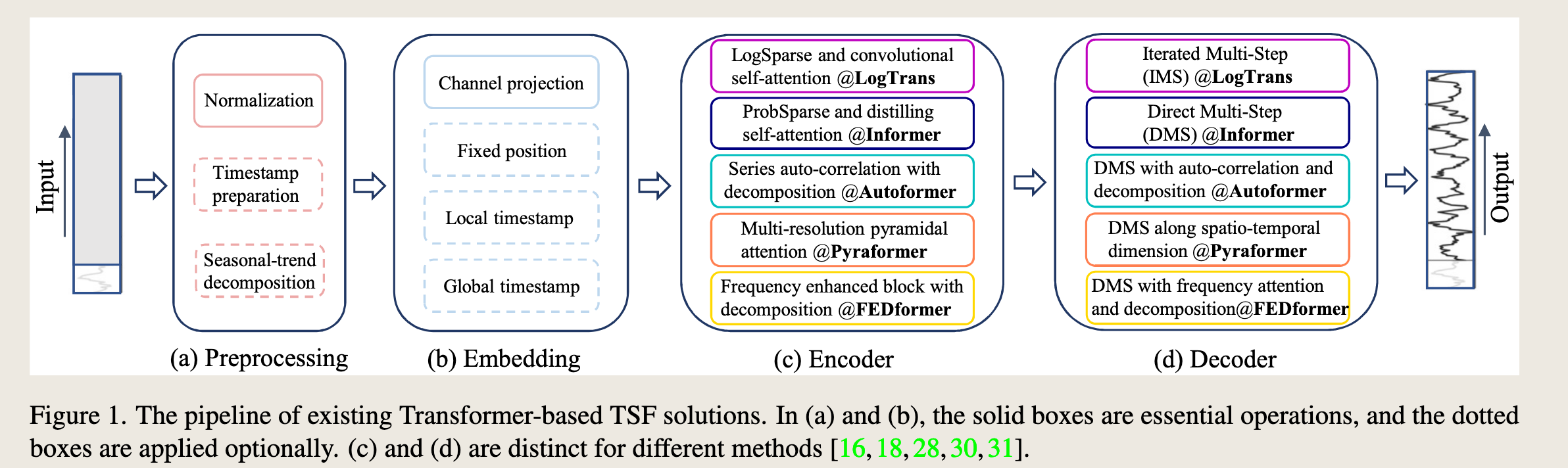
图 1 展示了现有的基于 Transformer 的时间序列预测（TSF）解决方案的流程。整个流程分为四个主要阶段：预处理（Preprocessing）、嵌入（Embedding）、编码器（Encoder）和解码器（Decoder）。

(a) 预处理（Preprocessing）： - 包括归一化（Normalization）和时间戳准备（Timestamp preparation）。 - 可选操作有季节趋势分解（Seasonal-trend decomposition）。

(b) 嵌入（Embedding）： - 包括通道投影（Channel projection）和固定位置编码（Fixed position）。 - 可选操作有本地时间戳（Local timestamp）和全局时间戳（Global timestamp）。

(c) 编码器（Encoder）： - 包括 LogSparse 和卷积自注意力（LogSparse and convolutional self-attention @LogTrans）。 - 包括 ProbSparse 和蒸馏自注意力（ProbSparse and distilling self-attention @Informer）。 - 包括序列自相关与分解（Series auto-correlation with decomposition @Autoformer）。 - 包括多分辨率金字塔注意力（Multi-resolution pyramidal attention @Pyraformer）。 - 包括频率增强块与分解（Frequency enhanced block with decomposition @FEDformer）。

(d) 解码器（Decoder）： - 包括迭代多步（IMS）预测（Iterated Multi-Step (IMS) @LogTrans）。 - 包括直接多步（DMS）预测（Direct Multi-Step (DMS) @Informer）。 - 包括 DMS 与自相关和分解（DMS with auto-correlation and decomposition @Autoformer）。 - 包括 DMS 沿时空维度（DMS along spatio-temporal dimension @Pyraformer）。 - 包括 DMS 与频率注意力和分解（DMS with frequency attention and decomposition @FEDformer）。

图中实线框表示基本操作，虚线框表示可选操作。(c) 和 (d) 部分针对不同的方法有不同的实现方式，分别对应文献 [16, 18, 28, 30, 31] 中的方法。

已经证明了并行多步预测效果更好

4. An Embarrassingly Simple Baseline¶

In the experiments of existing Transformer-based LTSF solutions ($T \gg 1$), all the compared (non-Transformer) baselines are IMS forecasting techniques, which are known to suffer from significant error accumulation effects. We hypothesize that the performance improvements in these works are largely due to the DMS strategy used in them.

在现有的基于Transformer的长期时间序列预测（LTSF）解决方案（$T \gg 1$）的实验中，所有比较的（非Transformer）基线都是迭代多步（IMS）预测技术，这些技术已知会遭受显著的误差累积效应。我们假设这些工作中的性能提升主要是由于其中使用的直接多步（DMS）策略。

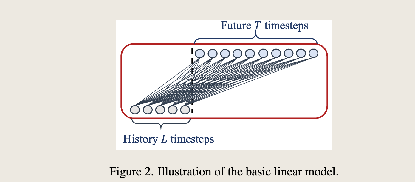
To validate this hypothesis, we present the simplest DMS model via a temporal linear layer, named LTSF-Linear, as a baseline for comparison.

The basic formulation of LTSF-Linear directly regresses historical time series for future prediction via a weighted sum operation (as illustrated in Figure 2).

The mathematical expression is $\hat{X}_i = W X_i$, where $W \in \mathbb{R}^{T \times L}$ is a linear layer along the temporal axis. $\hat{X}_i$ and $X_i$ are the prediction and input for each $i^{th}$ variate. Note that LTSF-Linear shares weights across different variates and does not model any spatial correlations.

为了验证这一假设，我们通过一个时间线性层提出了最简单的直接多步（DMS）模型，命名为LTSF-Linear，作为比较的基线。LTSF-Linear的基本公式直接通过加权求和操作回归历史时间序列以进行未来预测（如图2所示）。数学表达式为 $\hat{X}_i = W X_i$，其中 $W \in \mathbb{R}^{T \times L}$ 是沿时间轴的线性层。$\hat{X}_i$ 和 $X_i$ 分别是每个第 $i$ 个变量的预测和输入。请注意，LTSF-Linear在不同变量之间共享权重，并且不建模任何空间相关性。

LTSF-Linear is a set of linear models. Vanilla Linear is a one-layer linear model. To handle time series across different domains (e.g., finance, traffic, and energy domains), we further introduce two variants with two preprocessing methods, named DLinear and NLinear.

LTSF-Linear是一组线性模型。其中，Vanilla Linear是一个单层线性模型。为了处理不同领域（例如金融、交通和能源领域）的时间序列，我们进一步引入了两种预处理方法的两个变体，分别命名为DLinear和NLinear。

Specifically, DLinear is a combination of a Decomposition scheme used in Autoformer and FEDformer with linear layers. It first decomposes a raw data input into a trend component by a moving average kernel and a remainder (seasonal) component. Then, two one-layer linear layers are applied to each component, and we sum up the two features to get the final prediction. By explicitly handling trend, DLinear enhances the performance of a vanilla linear when there is a clear trend in the data.

具体来说，DLinear是结合了Autoformer和FEDformer中使用的分解方案与线性层的组合。它首先通过移动平均核将原始数据输入分解为趋势成分和剩余（季节性）成分。然后，对每个成分应用两个单层线性层，并将两个特征相加以获得最终预测。通过明确处理趋势，当数据中存在明显趋势时，DLinear增强了普通线性模型的性能。

序列分解有用

Meanwhile, to boost the performance of LTSF-Linear when there is a distribution shift in the dataset, NLinear first subtracts the input by the last value of the sequence. Then, the input goes through a linear layer, and the subtracted part is added back before making the final prediction. The subtraction and addition in NLinear are a simple normalization for the input sequence.

同时，为了在数据集中出现分布偏移时提升LTSF-Linear的性能，NLinear首先将输入序列的最后一个值从输入中减去。然后，输入经过一个线性层，最后在做出最终预测前将减去的部分加回。NLinear中的减法和加法是对输入序列进行的一种简单归一化处理。

减去最后一个值，减少分布偏移

5. Experiments¶

所以说这篇论文一定要读读，因为它都没有method 部分，做了很多实验

5.1. Experimental Settings¶

Dataset. We conduct extensive experiments on nine widely-used real-world datasets, including ETT (Electricity Transformer Temperature) [30] (ETTh1, ETTh2, ETTm1, ETTm2), Traffic, Electricity, Weather, ILI, ExchangeRate [15]. All of them are multivariate time series. We leave data descriptions in the Appendix.

公共数据集上的实验

Evaluation metric. Following previous works [28, 30, 31], we use Mean Squared Error (MSE) and Mean Absolute Error (MAE) as the core metrics to compare performance.

Compared methods. We include five recent Transformer-based methods: FEDformer [31], Autoformer [28], Informer [30], Pyraformer [18], and LogTrans [16]. Besides, we include a naive DMS method: Closest Repeat (Repeat), which repeats the last value in the look-back window, as another simple baseline. Since there are two variants of FEDformer, we compare the one with better accuracy (FEDformer-f via Fourier transform).

比较方法。 我们纳入了五种近期的基于Transformer的方法：FEDformer[31]、Autoformer[28]、Informer[30]、Pyraformer[18]和LogTrans[16]。此外，我们还包含了一种简单的直接多步（DMS）方法：Closest Repeat（Repeat），该方法通过重复回溯窗口中的最后一个值来作为另一个简单的基线。由于FEDformer有两种变体，我们比较的是准确度更高的那一种（通过傅里叶变换的FEDformer-f）。

5.2. Comparison with Transformers¶

Quantitative results. In Table 2, we extensively evaluate all mentioned Transformers on nine benchmarks, following the experimental setting of previous work [28, 30, 31]. Surprisingly, the performance of LTSF-Linear surpasses the SOTA FEDformer in most cases by 20% ∼ 50% improvements on the multivariate forecasting, where LTSFLinear even does not model correlations among variates. For different time series benchmarks, NLinear and DLinear show the superiority to handle the distribution shift and trend-seasonality features. We also provide results for univariate forecasting of ETT datasets in the Appendix, where LTSF-Linear still consistently outperforms Transformerbased LTSF solutions by a large margin.

定量结果。 在表2中，我们根据之前工作[28, 30, 31]的实验设置，对所有提到的Transformer模型在九个基准数据集上进行了广泛的评估。令人惊讶的是，LTSF-Linear在大多数情况下的性能超过了最先进的FEDformer，其在多变量预测上的改进幅度达到了20%至50%，尽管LTSF-Linear甚至没有对变量之间的相关性进行建模。对于不同的时间序列基准测试，NLinear和DLinear显示出在处理分布偏移和趋势季节性特征方面的优越性。我们还在附录中提供了ETT数据集的单变量预测结果，其中LTSF-Linear仍然以较大优势持续超越基于Transformer的LTSF解决方案。

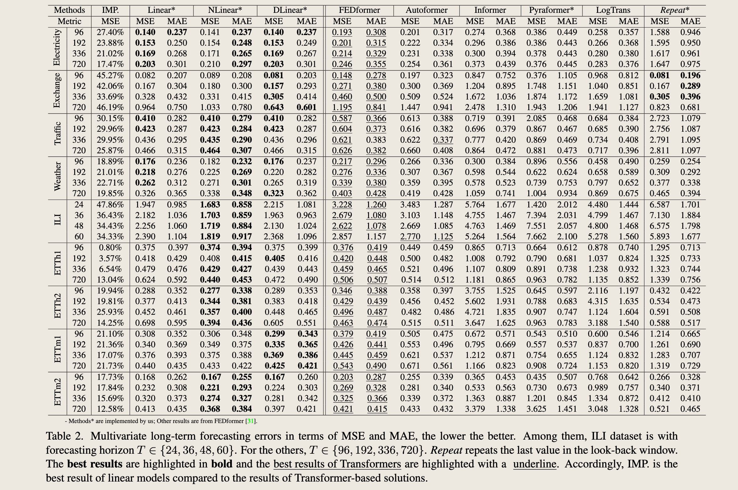
表2. 多变量长期预测误差以均方误差（MSE）和平均绝对误差（MAE）表示，数值越低越好。其中，ILI数据集的预测范围 $T$ 属于 $\{24, 36, 48, 60\}$。对于其他数据集，$T$ 属于 $\{96, 192, 336, 720\}$。Repeat方法通过重复回溯窗口中的最后一个值来进行预测。最佳结果以粗体显示，而基于Transformer的最佳结果则以下划线标出。相应地，IMP.表示与基于Transformer的解决方案相比，线性模型的最佳结果。

FEDformer achieves competitive forecasting accuracy on ETTh1. This because FEDformer employs classical time series analysis techniques such as frequency processing, which brings in time series inductive bias and benefits the ability of temporal feature extraction. In summary, these results reveal that existing complex Transformer-based LTSF solutions are not seemingly effective on the existing nine benchmarks while LTSF-Linear can be a powerful baseline.

FEDformer在ETTh1数据集上取得了有竞争力的预测准确性。这是因为FEDformer采用了诸如频率处理等经典的时间序列分析技术，这些技术引入了时间序列的归纳偏好，并有助于时间特征提取的能力。总结来说，这些结果揭示了现有的复杂基于Transformer的长期时间序列预测（LTSF）解决方案在现有的九个基准测试中似乎并不十分有效，而LTSF-Linear可以成为一个强大的基线模型。

Another interesting observation is that even though the naive Repeat method shows worse results when predicting long-term seasonal data (e.g., Electricity and Traffic), it surprisingly outperforms all Transformer-based methods on Exchange-Rate (around 45%). This is mainly caused by the wrong prediction of trends in Transformer-based solutions, which may overfit toward sudden change noises in the training data, resulting in significant accuracy degradation (see Figure 3(b)). Instead, Repeat does not have the bias.

另一个有趣的观察是，尽管朴素的Repeat方法在预测长期季节性数据（例如，电力和交通）时表现更差，但它在汇率（Exchange-Rate）上意外地优于所有基于Transformer的方法（大约45%）。这主要是由于基于Transformer的解决方案对趋势的错误预测，这些解决方案可能过度拟合训练数据中突然变化的噪声，导致显著的准确性下降（见图3(b)）。相反，Repeat方法没有这种偏差。

Qualitative results. As shown in Figure 3, we plot the prediction results on three selected time series datasets with Transformer-based solutions and LTSF-Linear: Electricity (Sequence 1951, Variate 36), Exchange-Rate (Sequence 676, Variate 3), and ETTh2 ( Sequence 1241, Variate 2), where these datasets have different temporal patterns.

When the input length is 96 steps, and the output horizon is 336 steps, Transformers [28, 30, 31] fail to capture the scale and bias of the future data on Electricity and ETTh2.

Moreover, they can hardly predict a proper trend on aperiodic data such as Exchange-Rate.

These phenomena further indicate the inadequacy of existing Transformer-based solutions for the LTSF task.

定性结果。 如图3所示，我们绘制了三个选定时间序列数据集的预测结果，这些数据集具有不同的时间模式：电力（Sequence 1951, Variate 36）、汇率（Sequence 676, Variate 3）和ETTh2（Sequence 1241, Variate 2），并将其与基于Transformer的解决方案和LTSF-Linear进行比较。当输入长度为96步，输出范围为336步时，Transformers[28, 30, 31]未能捕捉到电力和ETTh2数据的规模和偏差。此外，它们几乎无法预测诸如汇率这样的非周期性数据的适当趋势。这些现象进一步表明现有基于Transformer的解决方案对于长期时间序列预测（LTSF）任务的不足。

5.3. More Analyses on LTSF-Transformers¶

这部分的脉络：

Can existing LTSF-Transformers extract temporal relations well from longer input sequences? 回溯窗口的长度
What can be learned for long-term forecasting?（close input&far input）
Are the self-attention scheme effective for LTSF?复杂的自注意力机制是否有用
Can existing LTSF-Transformers preserve temporal order well?现有的 Transformer 模型是否保存了时间顺序
How effective are different embedding strategies?嵌入策略的讨论
Is training data size a limiting factor for existing LTSFTransformers?训练数据集的规模大小是否对模型有显著影响
Is efficiency really a top-level priority?

作者提出了 6 个问题，并且分别进行实验

(1)回溯窗口的长度¶

Can existing LTSF-Transformers extract temporal relations well from longer input sequences?

The size of the look-back window greatly impacts forecasting accuracy as it determines how much we can learn from historical data. Generally speaking, a powerful TSF model with a strong temporal relation extraction capability should be able to achieve better results with larger look-back window sizes.

现有的基于Transformer的长期时间序列预测（LTSF）模型能否很好地从较长的输入序列中提取时间关系？

回溯窗口的大小对预测准确性有很大影响，因为它决定了我们可以从历史数据中学到多少。一般来说，一个强大的时间序列预测（TSF）模型如果具有强大的时间关系提取能力，应该能够在更大的回溯窗口尺寸下取得更好的结果。然而，现有研究表明，当回溯窗口尺寸增大时，基于Transformer的模型的性能会恶化或保持稳定。这进一步表明现有基于Transformer的解决方案对于长期时间序列预测（LTSF）任务的不足。

To study the impact of input look-back window sizes, we conduct experiments with $L \in \{24, 48, 72, 96, 120, 144, 168, 192, 336, 504, 672, 720\}$ for long-term forecasting ($T=720$).

Figure 4 demonstrates the MSE results on two datasets.

Similar to the observations from previous studies [27, 30], existing Transformer-based models’ performance deteriorates or stays stable when the look-back window size increases.

In contrast, the performances of all LTSF-Linear are significantly boosted with the increase of look-back window size. Thus, existing solutions tend to overfit temporal noises instead of extracting temporal information if given a longer sequence, and the input size 96 is exactly suitable for most Transformers.

为了研究输入回溯窗口大小的影响，我们针对长期预测 ($T=720$) 进行了 $L \in \{24, 48, 72, 96, 120, 144, 168, 192, 336, 504, 672, 720\}$ 的实验。图4展示了两个数据集上的MSE结果。与之前研究[27, 30]的观察结果相似，现有的基于Transformer的模型在回溯窗口大小增加时性能会恶化或保持稳定。相比之下，所有LTSF-Linear的性能随着回溯窗口大小的增加而显著提升。

因此，现有的解决方案在给定更长序列时往往会过度拟合时间噪声，而不是提取时间信息，输入大小96对于大多数Transformer来说恰好合适。

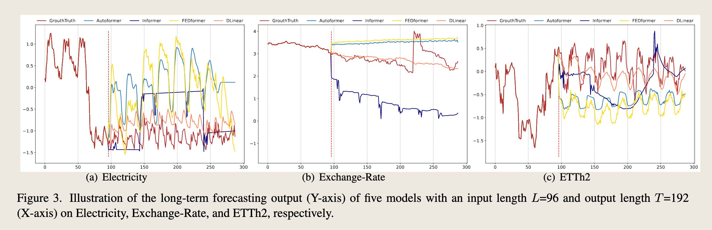
图3展示了五个模型在三个不同时间序列数据集上的长期预测输出（Y轴）与真实值（GrowthTruth）的对比。这些数据集分别是电力（Electricity）、汇率（Exchange-Rate）和ETTh2。X轴代表时间序列的索引。

电力（Electricity）：在电力数据集上，DLinear模型（黄色线）和FEDformer（黄色线）的预测结果与真实值（红色线）较为接近，尤其是在预测的前半部分。Informer（蓝色线）和Autoformer（浅蓝色线）的预测结果在某些区域偏离真实值较大。
汇率（Exchange-Rate）：在汇率数据集上，DLinear模型（黄色线）的预测结果与真实值（红色线）最为接近，尤其是在预测的后半部分。FEDformer（黄色线）和Informer（蓝色线）的预测结果在某些区域偏离真实值较大。
ETTh2：在ETTh2数据集上，DLinear模型（黄色线）的预测结果与真实值（红色线）较为接近，尤其是在预测的中间部分。Informer（蓝色线）和Autoformer（浅蓝色线）的预测结果在某些区域偏离真实值较大。

总体来看，DLinear模型在这三个数据集上的预测结果与真实值最为接近，表现出较好的预测性能。而其他基于Transformer的模型（如Informer、Autoformer和FEDformer）在某些区域的预测结果与真实值存在较大偏差。这表明在这些特定的时间序列数据集上，DLinear模型可能更适合捕捉数据的时间依赖关系。

Additionally, we provide more quantitative results in the Appendix, and our conclusion holds in almost all cases.

此外，我们在附录中提供了更定量的结果，并且在几乎所有情况下我们的结论都会得出。

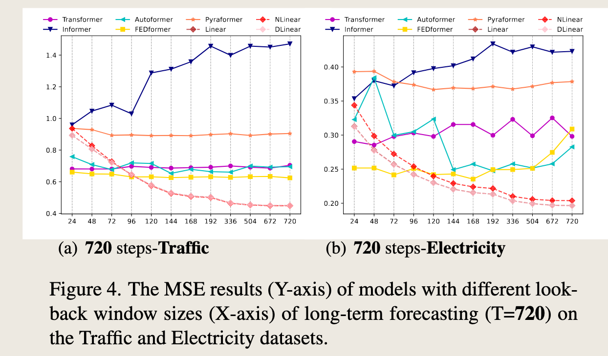
图4展示了不同模型在交通（Traffic）和电力（Electricity）数据集上进行长期预测（$T=720$步）时的均方误差（MSE）结果。X轴表示不同的回溯窗口大小，Y轴表示MSE值，数值越低表示预测性能越好。

(a) 720步-交通： - 该图显示了在交通数据集上，随着回溯窗口大小的增加，不同模型的MSE变化情况。 - 从图中可以看出，大多数基于Transformer的模型（如Informer、Autoformer、Pyraformer和FEDformer）的MSE随着窗口大小的增加而增加或保持稳定，这表明这些模型在处理更长的序列时可能会过拟合时间噪声，而不是提取时间信息。 - 相比之下，LTSF-Linear模型（包括NLinear和DLinear）的MSE随着窗口大小的增加而显著降低，显示出更好的性能提升。

(b) 720步-电力： - 该图显示了在电力数据集上，不同模型的MSE随回溯窗口大小的变化情况。 - 同样，基于Transformer的模型（如Informer、Autoformer、Pyraformer和FEDformer）的MSE在窗口大小增加时表现不稳定或增加。 - LTSF-Linear模型（包括NLinear和DLinear）在不同窗口大小下的表现相对稳定，并且在某些窗口大小下表现出显著的性能提升。

总体而言，这些结果表明，现有的基于Transformer的解决方案在处理长期预测任务时可能不如LTSF-Linear模型有效，特别是在回溯窗口较大的情况下。LTSF-Linear模型能够更好地利用更长的历史数据来提高预测准确性。

(2)close input & far input¶

What can be learned for long-term forecasting? While the temporal dynamics in the look-back window significantly impact the forecasting accuracy of short-term time series forecasting, we hypothesize that long-term forecasting depends on whether models can capture the trend and periodicity well only. That is, the farther the forecasting horizon, the less impact the look-back window itself has.

长期预测的启示： 尽管回溯窗口中的时间动态对短期时间序列预测的准确性有显著影响，但我们假设长期预测仅依赖于模型是否能够很好地捕捉趋势和周期性。也就是说，预测范围越远，回溯窗口本身的影响就越小。

em我也以为回溯窗口越长，预测准确性越高，可实验结果却好好像是，如果回溯窗口太长，无关信息造成的冗余信息越多，反而越来越学不到有用的信息。时序数据峰值数据可能占了更多的权重

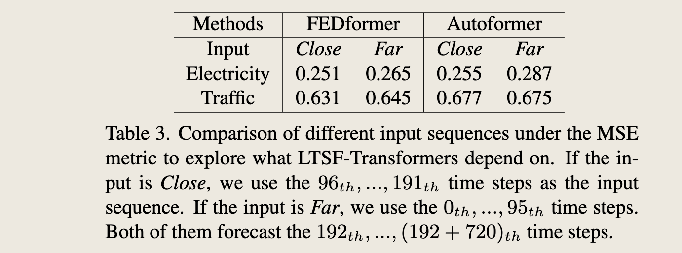
图3展示了FEDformer和Autoformer两种模型在不同输入序列（Close和Far）下的均方误差（MSE）比较，用于探索长期时间序列预测（LTSF）模型依赖于哪些输入序列。表中列出了两种模型在电力（Electricity）和交通（Traffic）数据集上的表现。

Close输入：指的是使用时间序列中较近的时间步（例如，对于电力数据集是第 $96_{th}$ 到 $191_{th}$ 时间步）作为输入序列。
Far输入：指的是使用时间序列中较远的时间步（例如，对于电力数据集是第 $0_{th}$ 到 $95_{th}$ 时间步）作为输入序列。
两种输入序列都预测从第 $192_{th}$ 时间步开始的未来 $720$ 个时间步。

从表中可以看出： - 在电力数据集上，无论是Close还是Far输入，FEDformer的MSE都略低于Autoformer，表明FEDformer在处理电力数据时表现稍好。 - 在交通数据集上，当输入为Close时，FEDformer和Autoformer的MSE相近；但当输入为Far时，Autoformer的MSE明显高于FEDformer，表明FEDformer在处理远端输入时具有更好的性能。

总体而言，这些结果表明，对于长期预测任务，输入序列的选择对模型性能有显著影响。特别是，FEDformer在处理远端输入时表现出更好的鲁棒性。

说明频域信息有用

To validate the above hypothesis, in Table 3, we compare the forecasting accuracy for the same future 720 time steps with data from two different look-back windows: (i). the original input L=96 setting (called Close) and (ii). the far input L=96 setting (called Far) that is before the original 96 time steps. From the experimental results, the performance of the SOTA Transformers drops slightly, indicating these models only capture similar temporal information from the adjacent time series sequence. Since capturing the intrinsic characteristics of the dataset generally does not require a large number of parameters, i,e. one parameter can represent the periodicity. Using too many parameters will even cause overfitting, which partially explains why LTSFLinear performs better than Transformer-based methods.

为了验证上述假设，在表3中，我们比较了使用两种不同回溯窗口数据预测相同未来720个时间步的准确性：

(i) 原始输入设置 $L=96$（称为Close）和

(ii) 远端输入设置 $L=96$（称为Far），即在原始96个时间步之前的设置。

从实验结果来看，最先进的Transformer模型的性能略有下降，这表明这些模型仅从相邻的时间序列中捕获了类似的时间信息。由于捕获数据集的内在特征通常不需要大量的参数，即一个参数就可以代表周期性。使用过多的参数甚至会导致过拟合，这在一定程度上解释了为什么LTSF-Linear的性能优于基于Transformer的方法。

嗯！

models only capture similar temporal information from the adjacent time series sequence

相邻时间序列捕获相同的趋势。所以直觉上以为，油温和温度、湿度有关的影响反而不大，反而带来更多的噪声

(3)自注意力机制是否有用¶

Are the self-attention scheme effective for LTSF?

We verify whether these complex designs in the existing Transformer (e.g., Informer) are essential. In Table 4, we gradually transform Informer to Linear. First, we replace each self-attention layer by a linear layer, called Att.-Linear, since a self-attention layer can be regarded as a fullyconnected layer where weights are dynamically changed. Furthermore, we discard other auxiliary designs (e.g., FFN) in Informer to leave embedding layers and linear layers, named Embed + Linear. Finally, we simplify the model to one linear layer. Surprisingly, the performance of Informer grows with the gradual simplification, indicating the unnecessary of the self-attention scheme and other complex modules at least for existing LTSF benchmarks.

自注意力机制是否对长期时间序列预测（LTSF）有效？

我们通过实验验证现有Transformer模型（例如Informer）中这些复杂设计的必要性。在表4中，我们逐步将Informer转变为线性模型。首先，我们用线性层替换每个自注意力层，称为Att.-Linear，因为自注意力层可以被视为权重动态变化的全连接层。此外，我们丢弃Informer中的其他辅助设计（例如，FFN），仅保留嵌入层和线性层，命名为Embed + Linear。最后，我们将模型简化为一个线性层。令人惊讶的是，随着模型的逐步简化，Informer的性能反而提高，这表明至少对于现有的LTSF基准测试，自注意力机制和其他复杂模块是不必要的。

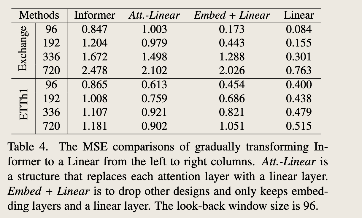
图4中的表格展示了将Informer模型逐步简化为线性模型的过程中，不同模型在两个数据集（Exchange和ETTh1）上的均方误差（MSE）比较。表格中的列分别代表不同的模型变体，行代表不同的回溯窗口大小。具体来说：

Informer：原始的基于Transformer的模型。
Att.-Linear：用线性层替换每个自注意力层的模型，因为自注意力层可以被视为权重动态变化的全连接层。
Embed + Linear：去掉Informer中的其他辅助设计（例如前馈神经网络，FFN），仅保留嵌入层和线性层。
Linear：进一步简化为单一线性层的模型。

表格中的数据展示了随着模型从左到右逐步简化，MSE的变化情况。可以观察到以下几点：

性能提升：随着模型的简化，Informer的性能在某些情况下有所提升，特别是在ETTh1数据集上，简化后的模型（Embed + Linear和Linear）表现出更低的MSE。
简化的有效性：在Exchange数据集上，简化后的模型（Embed + Linear和Linear）在较大的回溯窗口（336和720）下表现出更好的性能，而在较小的回溯窗口（96和192）下，原始Informer模型的性能略好。
自注意力机制的必要性：这些结果表明，对于现有的长期时间序列预测（LTSF）基准测试，自注意力机制和其他复杂模块可能并不是必需的。简化后的模型在某些情况下能够提供更好的预测性能。

总结来说，这些结果挑战了现有Transformer模型在长期时间序列预测任务中的必要性和有效性，表明简单的线性模型在某些情况下可能更为有效。

啊？也许模型并不是越复杂越好

(4)位置信息的保留¶

Can existing LTSF-Transformers preserve temporal order well?

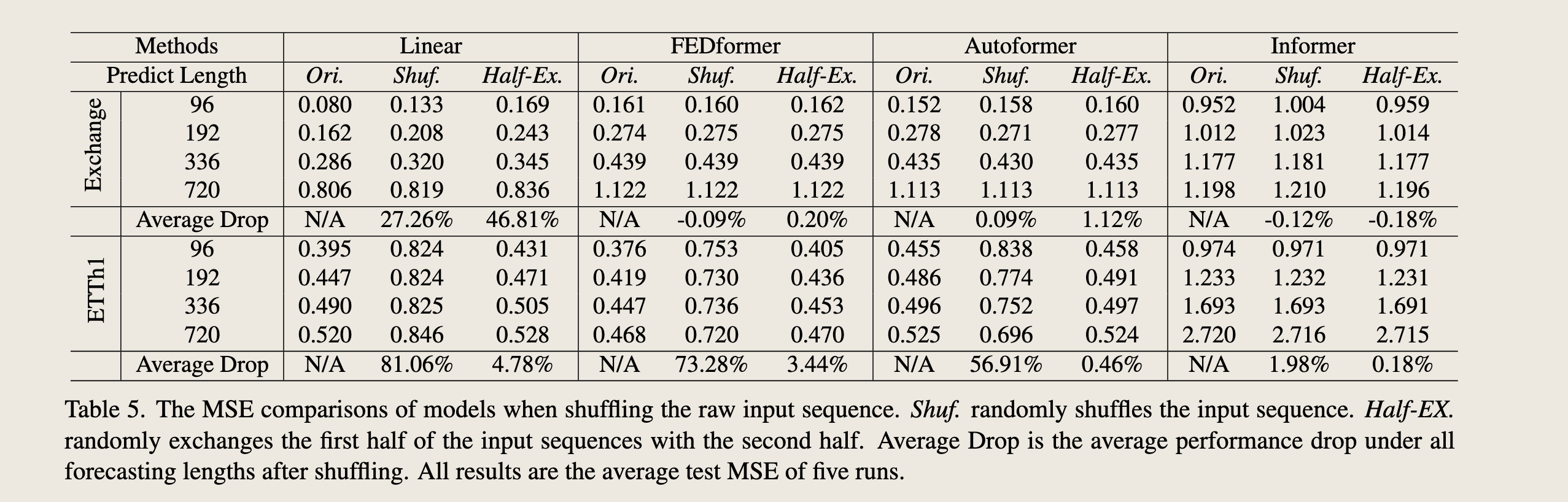
该图片展示了一张表格，标题为“Table 5. The MSE comparisons of models when shuffling the raw input sequence.” 表格比较了不同模型在输入序列被打乱时的平均均方误差（MSE）。具体来说，表格中列出了四种不同的打乱策略：原始序列（Ori.）、随机打乱（Shuf.）、半交换（Half-Ex.），以及在这些打乱策略下模型的性能表现。

表格中包含的模型有： - Linear（线性模型） - FEDformer - Autoformer - Informer

预测长度（Predict Length）分为四个不同的值：96、192、336、720。

对于每个模型和预测长度，表格展示了在不同打乱策略下的平均MSE值。此外，还计算了每种打乱策略相对于原始序列（Ori.）的平均性能下降百分比（Average Drop）。

从表格中可以观察到： - 线性模型（Linear）在所有预测长度下，随机打乱（Shuf.）和半交换（Half-Ex.）策略下的性能下降百分比最大，分别为27.26%和46.81%（对于Exchange Rate数据集）以及81.06%和4.78%（对于ETTh1数据集）。 - FEDformer和Autoformer在随机打乱（Shuf.）策略下的性能下降百分比相对较小，分别为-0.09%和0.09%（对于Exchange Rate数据集）以及73.28%和56.91%（对于ETTh1数据集）。 - Informer模型在所有打乱策略下的性能下降百分比最小，分别为-0.12%和-0.18%（对于Exchange Rate数据集）以及1.98%和0.18%（对于ETTh1数据集）。

表格底部的注释说明了这些结果是基于五次运行的平均测试MSE得出的。总体来看，Informer模型在处理打乱的输入序列时表现更为稳健，而线性模型的性能下降最为显著。

Self-attention is inherently permutation invariant, i.e., regardless of the order.

However, in timeseries forecasting, the sequence order often plays a crucial role. We argue that even with positional and temporal embeddings, existing Transformer-based methods still suffer from temporal information loss.

（打乱策略）In Table 5, we shuffle the raw input before the embedding strategies.

Two shuffling strategies are presented: ① Shuf. randomly shuffles the whole input sequences and ② Half-Ex. exchanges the first half of the input sequence with the second half.

（打乱以后得实验结果）Interestingly, compared with the original setting (Ori.) on the Exchange Rate, the performance of all Transformer-based methods does not fluctuate even when the input sequence is randomly shuffled.

By contrary, the performance of LTSF-Linear is damaged significantly.

（讨论）These indicate that LTSF-Transformers with different positional and temporal embeddings preserve quite limited temporal relations and are prone to overfit on noisy financial data, while the LTSF-Linear can model the order naturally and avoid overfitting with fewer parameters.

自注意力机制本质上是排列不变的，即与顺序无关。然而，在时间序列预测中，序列顺序往往起着至关重要的作用。我们主张即使使用位置和时间嵌入，现有的基于Transformer的方法仍然存在时间信息丢失的问题。

在表5中，我们在嵌入策略之前对原始输入进行了随机打乱。我们提出了两种打乱策略：“Shuf.”随机打乱整个输入序列，“Half-Ex.”将输入序列的前半部分与后半部分进行交换。有趣的是，与汇率数据集的原始设置（“Ori.”）相比，即使输入序列被随机打乱，所有基于Transformer的方法的性能也没有波动。相比之下，LTSF-Linear的性能却受到了显著的损害。

这些结果表明，具有不同位置和时间嵌入的LTSF-Transformer保留的时间关系相当有限，且容易在嘈杂的金融数据上过拟合，而简单的LTSF-Linear能够自然地模拟顺序，并且由于参数较少而避免了过拟合。

For the ETTh1 dataset, FEDformer and Autoformer introduce time series inductive bias into their models, making them can extract certain temporal information when the dataset has more clear temporal patterns (e.g., periodicity) than the Exchange Rate.

Therefore, the average drops of the two Transformers are 73.28% and 56.91% under the Shuf. setting, where it loses the whole order information.

Moreover, Informer still suffers less from both Shuf. and Half-Ex. settings due to its no such temporal inductive bias. Overall, the average drops of LTSF-Linear are larger than Transformer-based methods for all cases, indicating the existing Transformers do not preserve temporal order well.

对于ETTh1数据集，FEDformer和Autoformer通过引入时间序列归纳偏置，使其能够在数据集具有更清晰的时间模式（例如周期性）时提取特定的时间信息，这比汇率数据集更具优势。

因此，在随机打乱（Shuf.）设置下，这两个Transformer的平均性能下降幅度分别为73.28%和56.91%，在这种情况下，整个顺序信息丢失。

此外，由于Informer没有这种时间归纳偏置，因此在随机打乱（Shuf.）和半交换（Half-Ex.）设置下受到的影响较小。总体而言，LTSF-Linear在所有情况下平均性能下降幅度都大于基于Transformer的方法，这表明现有的Transformer在保留时间顺序方面表现不佳。

(5)讨论不同的嵌入策略¶

How effective are different embedding strategies?

We study the benefits of position and timestamp embeddings used in Transformer-based methods. In Table 6, the forecasting errors of Informer largely increase without positional embeddings (wo/Pos.). Without timestamp embeddings (wo/Temp.) will gradually damage the performance of Informer as the forecasting lengths increase. Since Informer uses a single time step for each token, it is necessary to introduce temporal information in tokens.

不同的嵌入策略在Transformer模型中的效果如何？

我们研究了位置嵌入（positional embeddings）和时间戳嵌入（timestamp embeddings）在基于Transformer的方法中的效果。如表 6 所示，对于Informer模型而言，没有位置嵌入（wo/Pos.）的情况下，预测误差显著增加。没有时间戳嵌入（wo/Temp.）会随着预测长度的增加而逐渐损害Informer的性能。这是因为Informer每个token仅使用一个时间步长，因此在token中引入时间信息是必要的。

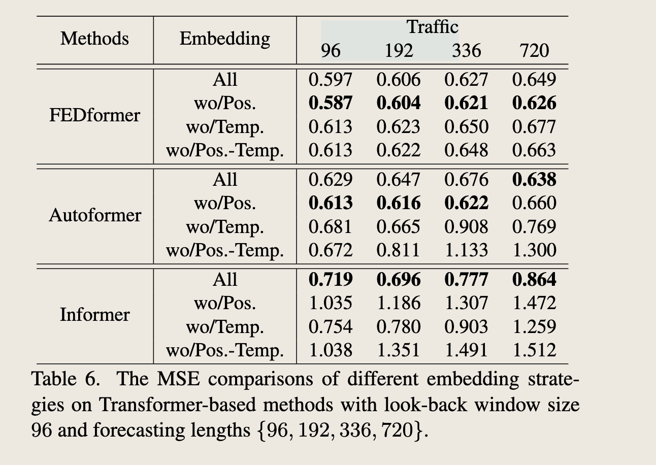
“Table 6. The MSE comparisons of different embedding strategies on Transformer-based methods with look-back window size 96 and forecasting lengths {96, 192, 336, 720}.”

表格比较了不同嵌入策略在基于Transformer的方法上的平均均方误差（MSE），这些方法使用96大小的回溯窗口，并在不同的预测长度（96、192、336、720）下进行测试。

表格中包含的模型有： - FEDformer - Autoformer - Informer

嵌入策略包括： - 使用所有嵌入（All） - 不使用位置嵌入（wo/Pos.） - 不使用时间戳嵌入（wo/Temp.） - 同时不使用位置和时间戳嵌入（wo/Pos.-Temp.）

对于每个模型和预测长度，表格展示了在不同嵌入策略下的平均MSE值。这些结果可以帮助我们理解位置嵌入和时间戳嵌入在不同模型中的重要性。

从表格中可以观察到： - 对于FEDformer模型，不使用位置嵌入（wo/Pos.）时，MSE值略有下降，而不使用时间戳嵌入（wo/Temp.）或同时不使用两者（wo/Pos.-Temp.）时，MSE值有所增加。 - 对于Autoformer模型，不使用位置嵌入（wo/Pos.）时，MSE值略有下降，而不使用时间戳嵌入（wo/Temp.）或同时不使用两者（wo/Pos.-Temp.）时，MSE值显著增加。 - 对于Informer模型，不使用位置嵌入（wo/Pos.）时，MSE值显著增加，而不使用时间戳嵌入（wo/Temp.）或同时不使用两者（wo/Pos.-Temp.）时，MSE值也显著增加，尤其是在较长的预测长度下。

位置嵌入和时间戳嵌入对于Informer模型的性能至关重要，而对于FEDformer和Autoformer模型，位置嵌入的影响较小，时间戳嵌入的影响较为显著。

Rather than using a single time step in each token, FEDformer and Autoformer input a sequence of timestamps to embed the temporal information. Hence, they can achieve comparable or even better performance without fixed positional embeddings. However, without timestamp embeddings, the performance of Autoformer declines rapidly because of the loss of global temporal information. Instead, thanks to the frequency-enhanced module proposed in FEDformer to introduce temporal inductive bias, it suffers less from removing any position/timestamp embeddings.

与每个token仅使用单一时间步长不同，FEDformer和Autoformer输入一系列时间戳来嵌入时间信息。因此，它们能够在没有固定位置嵌入的情况下实现可比甚至更好的性能。然而，如果没有时间戳嵌入，Autoformer的性能会因为失去全局时间信息而迅速下降。相反，由于FEDformer中提出的频率增强模块引入了时间归纳偏置，它在移除任何位置/时间戳嵌入时受到的影响较小。

作者好懂这些模型

(6)数据集的规模¶

Is training data size a limiting factor for existing LTSFTransformers? Some may argue that the poor performance of Transformer-based solutions is due to the small sizes of the benchmark datasets. Unlike computer vision or natural language processing tasks, TSF is performed on collected time series, and it is difficult to scale up the training data size. In fact, the size of the training data would indeed have a significant impact on the model performance. Accordingly, we conduct experiments on Traffic, comparing the performance of the model trained on a full dataset (17,544*0.7 hours), named Ori., with that trained on a shortened dataset (8,760 hours, i.e., 1 year), called Short.Unexpectedly, Table 7 presents that the prediction errors with reduced training data are lower in most cases. This might because the whole-year data maintains more clear temporal features than a longer but incomplete data size. While we cannot conclude that we should use less data for training, it demonstrates that the training data scale is not the limiting reason for the performances of Autoformer and FEDformer.

有人可能会认为基于Transformer的解决方案性能不佳是由于基准数据集的规模较小。与计算机视觉或自然语言处理任务不同，时间序列预测（TSF）是在收集到的时间序列上执行的，并且很难扩大训练数据的规模。实际上，训练数据的大小确实会对模型性能产生重大影响。因此，我们在Traffic数据集上进行了实验，比较了在完整数据集（17,544*0.7小时）上训练的模型（命名为Ori.）与在缩短数据集（8,760小时，即1年）上训练的模型（称为Short）的性能。出乎意料的是，表7显示，在大多数情况下，减少训练数据后的预测误差更低。这可能是因为全年数据比更长但不完整的数据集保持了更清晰的时间特征。虽然我们不能得出我们应该使用更少数据进行训练的结论，但它表明训练数据规模并不是Autoformer和FEDformer性能的限制原因。

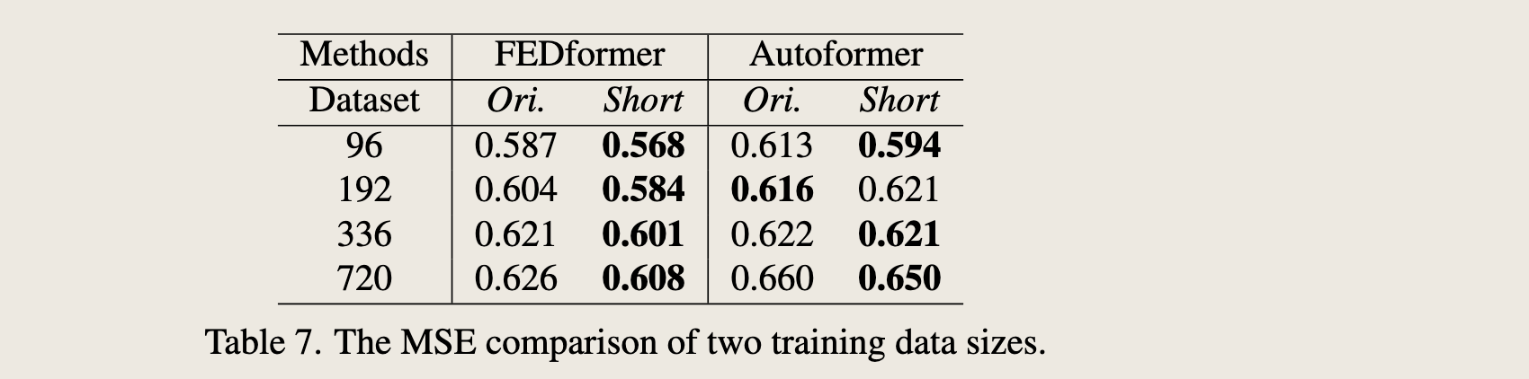
训练数据集规模变小但是预测效果更好了，因为虽然训练数据集变小了，但保存了完整的数据变化模式。

(7)效率真的很重要吗？¶

Is efficiency really a top-level priority?

Existing LTSF-Transformers claim that the $O(L^2)$ complexity of the vanilla Transformer is unaffordable for the LTSF problem.原始 Transformer 是平方级内存复杂度和时间复杂度

Although they prove to be able to improve the theoretical time and memory complexity from $O(L^2)$ to $O(L)$, it is unclear whether 1) the actual inference time and memory cost on devices are improved, and 2) the memory issue is unacceptable and urgent for today's GPU (e.g., an NVIDIA Titan XP here).

效率真的是最优先考虑的因素吗？现有的长序列时间序列预测Transformer（LTSF-Transformers）声称，传统Transformer的$O(L^2)$复杂度对于长序列时间序列预测（LTSF）问题来说是难以承受的。尽管它们证明了能够将理论时间和内存复杂度从$O(L^2)$改进到$O(L)$，但目前还不清楚1）设备上的实际推理时间和内存成本是否得到改善，以及2）内存问题是否是当前GPU（例如，这里的NVIDIA Titan XP）所不能接受且紧迫的。

In Table 8, we compare the average practical efficiencies with 5 runs. Interestingly, compared with the vanilla Transformer (with the same DMS decoder), most Transformer variants incur similar or even worse inference time and parameters in practice. These follow-ups introduce more additional design elements to make practical costs high. Moreover, the memory cost of the vanilla Transformer is practically acceptable, even for output length $L = 720$, which weakens the importance of developing a memory-efficient Transformers, at least for existing benchmarks.

在表8中，我们比较了5次运行的平均实际效率。有趣的是，与传统Transformer（使用相同的DMS解码器）相比，大多数Transformer变体在实践中产生了相似甚至更差的推理时间和参数。这些后续工作引入了更多的设计元素，使得实际成本变高。此外，即使对于输出长度$L = 720$，传统Transformer的内存成本在实践中也是可以接受的，这削弱了至少对于现有基准测试而言开发内存高效Transformer的重要性。

这篇论文出来，大家以后怎么研究时序呀，全面否定的程度

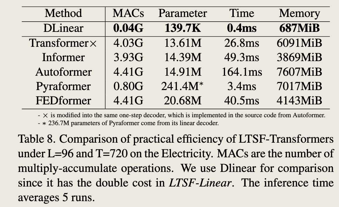
“Table 8. Comparison of practical efficiency of LTSF-Transformers under L=96 and T=720 on the Electricity.” 表格比较了在电力数据集上，预测长度L=96和时间步长T=720时，不同长序列时间序列预测（LTSF）Transformer模型的实际效率。效率通过四个指标来衡量：MACs（乘累加操作数）、参数数量、推理时间以及内存使用量。

表格中包含的模型有： - DLinear - Transformer×（修改自Autoformer的一步解码器） - Informer - Autoformer - Pyraformer - FEDformer

表格中的数据如下： - DLinear模型的MACs为0.04G，参数数量为139.K7，推理时间为0.4ms，内存使用量为687MiB。 - Transformer×模型的MACs为4.03G，参数数量为13.61M，推理时间为26.8ms，内存使用量为6091MiB。 - Informer模型的MACs为3.93G，参数数量为14.39M，推理时间为49.3ms，内存使用量为3869MiB。 - Autoformer模型的MACs为4.41G，参数数量为14.91M，推理时间为164.1ms，内存使用量为7607MiB。 - Pyraformer模型的MACs为0.80G，参数数量为241.4M*，推理时间为3.4ms，内存使用量为7017MiB。（注：Pyraformer的参数数量中236.7M来自其线性解码器） - FEDformer模型的MACs为4.41G，参数数量为20.68M，推理时间为40.5ms，内存使用量为4143MiB。

表格底部的注释说明： - Transformer×模型被修改为与Autoformer相同的一步解码器。 - Pyraformer模型的参数数量中，236.7M来自其线性解码器。 - 使用DLinear作为比较基准，因为它在LTSF-Linear中的成本是DLinear的两倍。 - 推理时间是5次运行的平均值。

总体来看，DLinear模型在所有指标上都表现出较高的效率，而Autoformer和FEDformer在内存使用量上较高，Informer在推理时间上最高。

该图片展示了一张表格，标题为“Table 8. Comparison of practical efficiency of LTSF-Transformers under L=96 and T=720 on the Electricity.” 表格比较了在电力数据集上，预测长度L=96和时间步长T=720时，不同长序列时间序列预测（LTSF）Transformer模型的实际效率。效率通过四个指标来衡量：MACs（乘累加操作数）、参数数量、推理时间以及内存使用量。

表格中包含的模型有： - DLinear - Transformer×（修改自Autoformer的一步解码器） - Informer - Autoformer - Pyraformer - FEDformer

表格中的数据如下： - DLinear模型的MACs为0.04G，参数数量为139.K7，推理时间为0.4ms，内存使用量为687MiB。 - Transformer×模型的MACs为4.03G，参数数量为13.61M，推理时间为26.8ms，内存使用量为6091MiB。 - Informer模型的MACs为3.93G，参数数量为14.39M，推理时间为49.3ms，内存使用量为3869MiB。 - Autoformer模型的MACs为4.41G，参数数量为14.91M，推理时间为164.1ms，内存使用量为7607MiB。 - Pyraformer模型的MACs为0.80G，参数数量为241.4M*，推理时间为3.4ms，内存使用量为7017MiB。（注：Pyraformer的参数数量中236.7M来自其线性解码器） - FEDformer模型的MACs为4.41G，参数数量为20.68M，推理时间为40.5ms，内存使用量为4143MiB。

表格底部的注释说明： - Transformer×模型被修改为与Autoformer相同的一步解码器。 - Pyraformer模型的参数数量中，236.7M来自其线性解码器。 - 使用DLinear作为比较基准，因为它在LTSF-Linear中的成本是DLinear的两倍。 - 推理时间是5次运行的平均值。

总体来看，DLinear模型在所有指标上都表现出较高的效率，而Autoformer和FEDformer在内存使用量上较高，Informer在推理时间上最高。

emm

6. Conclusion and Future Work¶

Conclusion. This work questions the effectiveness of emerging favored Transformer-based solutions for the longterm time series forecasting problem. We use an embarrassingly simple linear model LTSF-Linear as a DMS forecasting baseline to verify our claims. Note that our contributions do not come from proposing a linear model but rather from throwing out an important question, showing surprising comparisons, and demonstrating why LTSFTransformers are not as effective as claimed in these works through various perspectives. We sincerely hope our comprehensive studies can benefit future work in this area.

结论。本工作对新兴的基于Transformer的解决方案在长期时间序列预测问题上的有效性提出了质疑。我们使用一个极其简单的线性模型LTSF-Linear作为DMS预测的基线来验证我们的论断。需要注意的是，我们的贡献并非来自于提出一个线性模型，而是提出了一个重要的问题，展示了令人惊讶的比较结果，并从多个角度证明了为什么LTSF-Transformers并不像这些工作中所声称的那样有效。我们真诚地希望我们全面的研究所能为这一领域的未来工作带来益处。

现在 DLinear 又被很多模型对比，但也因此出现很多 Linear 系的文章，比如 UNetTSF

Future work. LTSF-Linear has a limited model capacity, and it merely serves a simple yet competitive baseline with strong interpretability for future research. For example, the one-layer linear network is hard to capture the temporal dynamics caused by change points [25]. Consequently, we believe there is a great potential for new model designs, data processing, and benchmarks to tackle the challenging LTSF problem.

未来工作。LTSF-Linear模型的容量有限，它仅作为一个简单但具有竞争力的基线，为未来的研究提供强有力的可解释性。例如，单层线性网络很难捕捉由变化点引起的时间动态。因此，我们相信在新模型设计、数据处理和基准测试方面，解决具有挑战性的长期时间序列预测（LTSF）问题具有巨大潜力。

Appendix¶

In this Appendix, we provide descriptions of non Transformer-based TSF solutions, detailed experimental settings, more comparisons under different look-back window sizes, and the visualization of LTSF-Linear on all datasets. We also append our code to reproduce the results shown in the paper.

在本附录中，我们提供了非Transformer基础的时间序列预测（TSF）解决方案的描述、详细的实验设置、在不同回溯窗口大小下的更多比较，以及LTSF-Linear在所有数据集上的可视化结果。我们还附上了重现论文中展示结果的代码。

As a long-standing problem with a wide range of applications, statistical approaches (e.g., autoregressive integrated moving average (ARIMA) [1], exponential smoothing [12], and structural models [14]) for time series forecasting have been used from the 1970s onward. Generally speaking, the parametric models used in statistical methods require significant domain expertise to build.

作为一个具有广泛应用的长期问题，自20世纪70年代以来，统计方法（例如，自回归积分滑动平均模型（ARIMA）[1]、指数平滑[12]和结构模型[14]）已被用于时间序列预测。一般来说，统计方法中使用的参数模型需要显著的领域专业知识来构建。

To relieve this burden, many machine learning techniques such as gradient boosting regression tree (GBRT) [10, 11] gain popularity, which learns the temporal dynamics of time series in a data-driven manner. However, these methods still require manual feature engineering and model designs. With the powerful representation learning capability of deep neural networks (DNNs) from abundant data, various deep learning-based TSF solutions are proposed in the literature, achieving better forecasting accuracy than traditional techniques in many cases.

为了减轻这一负担，许多机器学习技术，如梯度提升回归树（GBRT）[10, 11]，因其能够以数据驱动的方式学习时间序列的时间动态而变得流行。然而，这些方法仍然需要人工特征工程和模型设计。得益于深度神经网络（DNNs）的强大表示学习能力，从大量数据中，文献中提出了各种基于深度学习的TSF解决方案，在许多情况下比传统技术实现了更好的预测准确性。

Besides Transformers, the other two popular DNN architectures are also applied for time series forecasting:

除了Transformers，另外两种流行的DNN架构也被应用于时间序列预测：

其实是能感觉到的，深度学习设计的网络很少涉及专业知识，几乎不需要注入太多的专业知识，现在时序预测模型，设计深度学习的开始引入传统统计知识，比如序列分解，频域知识，刚开始的设计也不像是专门针对时序数据，但其实把具有长期趋势的成分剥离出来，不就是用 Transformer

Recurrent neural networks (RNNs) based methods (e.g., [21]) summarize the past information compactly in internal memory states and recursively update themselves for forecasting.
基于递归神经网络（RNNs）的方法（例如，[21]）在内部记忆状态中紧凑地总结过去信息，并递归地自我更新以进行预测。
Convolutional neural networks (CNNs) based methods (e.g., [3]), wherein convolutional filters are used to capture local temporal features.
基于卷积神经网络（CNNs）的方法（例如，[3]），其中使用卷积滤波器来捕捉局部时间特征。

RNN-based TSF methods belong to IMS forecasting techniques. Depending on whether the decoder is implemented in an autoregressive manner, there are either IMS or DMS forecasting techniques for CNN-based TSF methods [3, 17].

基于RNN的时间序列预测（TSF）方法属于单步预测（IMS）技术。根据解码器是否以自回归方式实现，对于基于CNN的TSF方法，可以是单步预测（IMS）或多步预测（DMS）技术[3, 17]。

B. Experimental Details¶

B.1. Data Descriptions¶

We use nine wildly-used datasets in the main paper. The details are listed in the following.

ETT (Electricity Transformer Temperature) [30]2 consists of two hourly-level datasets (ETTh) and two 15minute-level datasets (ETTm). Each of them contains seven oil and load features of electricity transformers from July 2016 to July 2018.
ETT（电力变压器温度）[30] 包含两个小时级别的数据集（ETTh）和两个15分钟级别的数据集（ETTm）。每个数据集都包含了从2016年7月至2018年7月的电力变压器的七个油和负载特征。
Traffic3 describes the road occupancy rates. It contains the hourly data recorded by the sensors of San Francisco freeways from 2015 to 2016.
交通[3] 描述了道路占用率。它包含了2015年至2016年旧金山高速公路传感器记录的每小时数据。
Electricity4 collects the hourly electricity consumption of 321 clients from 2012 to 2014.
电力[4] 收集了2012年至2014年321个客户的每小时电力消耗数据。
Exchange-Rate [15]5 collects the daily exchange rates of 8 countries from 1990 to 2016.
汇率[15] 收集了1990年至2016年8个国家的每日汇率。
Weather6 includes 21 indicators of weather, such as air temperature, and humidity. Its data is recorded every 10 min for 2020 in Germany.
天气[6] 包括21个气象指标，如空气温度和湿度。其数据是2020年在德国每10分钟记录一次的。
ILI7 describes the ratio of patients seen with influenzalike illness and the number of patients. It includes weekly data from the Centers for Disease Control and Prevention of the United States from 2002 to 2021.
ILI[7] 描述了患有流感样疾病的患者比例和患者数量。它包括了2002年至2021年美国疾病控制与预防中心的每周数据。

B.2. Implementation Details¶

For existing Transformer-based TSF solutions: the implementation of Autoformer [28], Informer [30], and the vanilla Transformer [26] are all taken from the Autoformer work [28]; the implementation of FEDformer [31] and Pyraformer [18] are from their respective code repository. We also adopt their default hyper-parameters to train the models. For DLinear, the moving average kernel size for decomposition is 25, which is the same as Autoformer. The total parameters of a vanilla linear model and a NLinear are TL. The total parameters of the DLinear are 2TL. Since LTSF-Linear will be underfitting when the input length is short, and LTSF-Transformers tend to overfit on a long lookback window size. To compare the best performance of existing LTSF-Transformers with LTSF-Linear, we report L=336 for LTSF-Linear and L=96 for Transformers by default. For more hyper-parameters of LTSF-Linear, please refer to our code.

对于现有的基于Transformer的时间序列预测（TSF）解决方案：Autoformer[28]、Informer[30]和传统Transformer[26]的实现都取自Autoformer的工作[28]；FEDformer[31]和Pyraformer[18]的实现分别来自它们各自的代码库。

我们还采用了它们的默认超参数来训练模型。对于DLinear，分解时移动平均核的大小为25，这与Autoformer相同。

一个传统线性模型和一个NLinear的总参数量为TL。DLinear的总参数量为2TL。

由于当输入长度较短时，LTSF-Linear可能会出现欠拟合，而LTSF-Transformers在较长的回溯窗口大小时则倾向于过拟合。为了比较现有LTSF-Transformers与LTSF-Linear的最佳性能，我们默认报告LTSF-Linear的L=336和Transformers的L=96。有关LTSF-Linear的更多超参数，请参阅我们的代码。

C. Additional Comparison with Transformers¶

We further compare LTSF-Linear with LTSFTransformer for Univariate Forecasting on four ETT datasets. Moreover, in Figure 4 of the main paper, we demonstrate that existing Transformers fail to exploit large look-back window sizes with two examples. Here, we give comprehensive comparisons between LTSF-Linear and Transformer-based TSF solutions under various look-back window sizes on all benchmarks.

我们进一步将LTSF-Linear与LTSF-Transformer在四个ETT数据集上进行单变量预测的比较。此外，在主要论文的图4中，我们通过两个例子展示了现有的Transformer无法利用大的回溯窗口大小。在此，我们在所有基准测试上，在各种回溯窗口大小下，对LTSF-Linear和基于Transformer的TSF解决方案进行了全面的比较。

C.1. Comparison of Univariate Forecasting¶

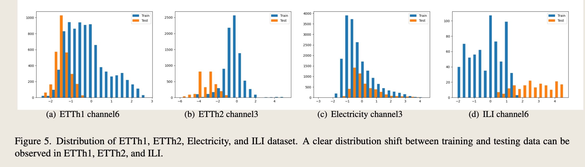
We present the univariate forecasting results on the four ETT datasets in table 9. Similarly, LTSF-Linear, especially for NLinear can consistently outperform all transformerbased methods by a large margin in most time. We find that there are serious distribution shifts between training and test sets (as shown in Fig. 5 (a), (b)) on ETTh1 and ETTh2 datasets. Simply normalization via the last value from the lookback window can greatly relieve the distribution shift problem.

我们在表9中展示了四个ETT数据集上的单变量预测结果。同样地，LTSF-Linear，特别是NLinear，在大多数情况下都能显著优于所有基于Transformer的方法。我们发现，在ETTh1和ETTh2数据集上，训练集和测试集之间存在严重的分布偏移（如图5(a)、(b)所示）。简单地通过回溯窗口的最后一个值进行归一化可以大大缓解分布偏移问题。

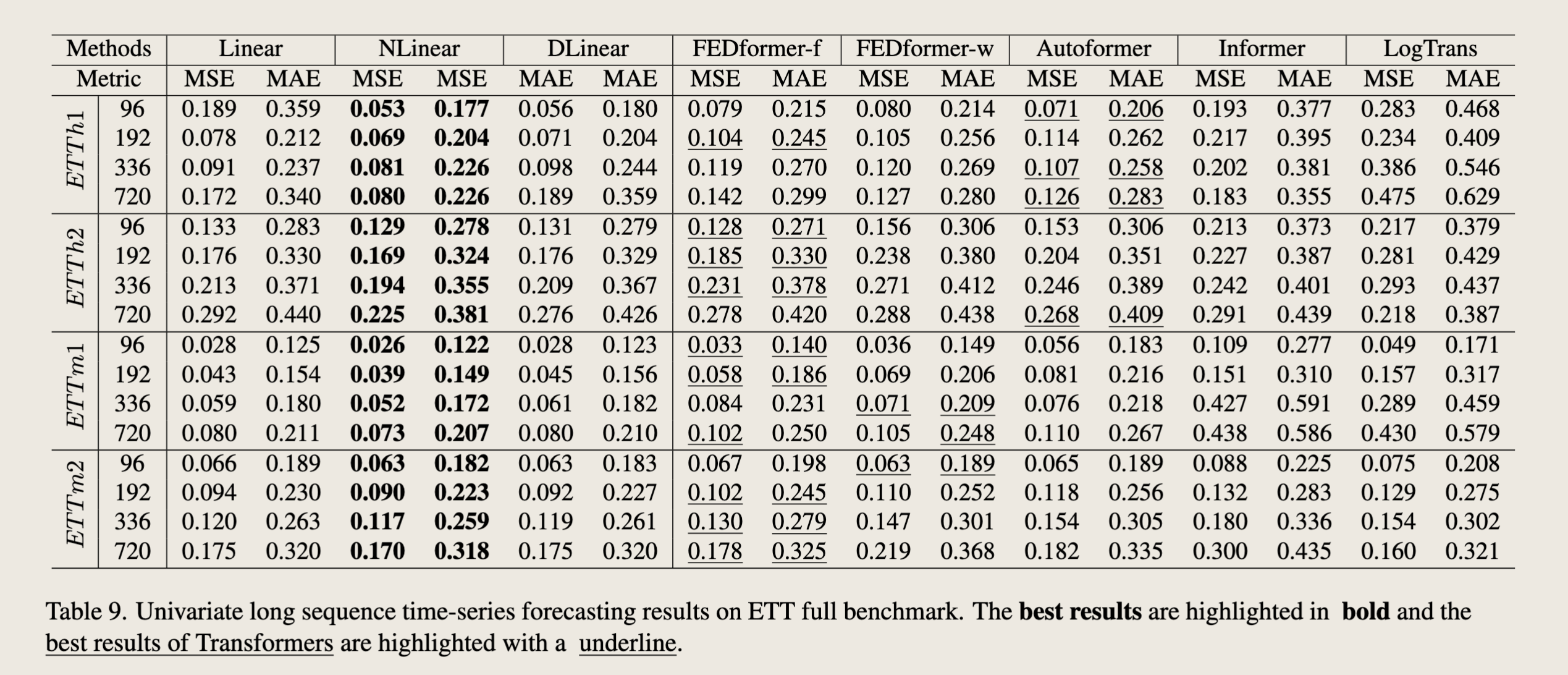
“Table 9. Univariate long sequence time-series forecasting results on ETT full benchmark.” 表格列出了在ETT完整基准测试上，不同模型在单变量长序列时间序列预测任务中的表现。表格中包含的模型有：

Linear（线性模型）
NLinear
DLinear
FEDformer-f
FEDformer-w
Autoformer
Informer
LogTrans

预测长度（Predict Length）分为四个不同的值：96、192、336、720。

对于每个模型和预测长度，表格展示了两种评价指标：均方误差（MSE）和平均绝对误差（MAE）。表格中用粗体字突出显示了最佳结果，而用下划线标出了Transformer模型的最佳结果。

从表格中可以观察到： - 在大多数情况下，DLinear模型在MSE和MAE指标上都取得了最佳性能。 - 在某些情况下，NLinear模型也取得了相对较好的性能，尤其是在ETTh1数据集的720预测长度下。 - 基于Transformer的模型（FEDformer、Autoformer、Informer、LogTrans）在某些情况下也表现良好，但通常不如DLinear和NLinear模型。 - Linear模型在所有情况下的性能都相对较差。

这些结果表明，在ETT数据集上的单变量长序列时间序列预测任务中，DLinear和NLinear模型通常比其他模型（包括基于Transformer的模型）表现更好。

ETT 数据集、Electricity 数据集、ILI 训练集&测试集上的分布偏移问题

C.2. Comparison under Different Look-back Windows¶

In Figure 6, we provide the MSE comparisons of five LTSF-Transformers with LTSF-Linear under different lookback window sizes to explore whether existing Transformers can extract temporal well from longer input sequences. For hourly granularity datasets (ETTh1, ETTh2, Traffic, and Electricity), the increasing look-back window sizes are {24, 48, 72, 96, 120, 144, 168, 192, 336, 504, 672, 720}, which represent {1, 2, 3, 4, 5, 6, 7, 8, 14, 21, 28, 30} days. The forecasting steps are {24, 720}, which mean {1, 30} days. For 5-minute granularity datasets (ETTm1 and ETTm2), we set the look-back window size as {24, 36, 48, 60, 72, 144, 288}, which represent {2, 3, 4, 5, 6, 12, 24} hours. For 10-minute granularity datasets (Weather), we set the look-back window size as {24, 48, 72, 96, 120, 144, 168, 192, 336, 504, 672, 720}, which mean {4, 8, 12, 16, 20, 24, 28, 32, 56, 84, 112, 120} hours. The forecasting steps are {24, 720} that are {4, 120} hours. For weekly granularity dataset (ILI), we set the look-back window size as {26, 52, 78, 104, 130, 156, 208}, which represent {0.5, 1, 1.5, 2, 2.5, 3, 3.5, 4} years. The corresponding forecasting steps are {26, 208}, meaning {0.5, 4} years.

在图6中，我们提供了五种LTSF-Transformer与LTSF-Linear在不同回溯窗口大小下的均方误差（MSE）比较，以探索现有的Transformer是否能够从更长的输入序列中很好地提取时间特征。对于小时粒度数据集（ETTh1、ETTh2、交通和电力），增加的回溯窗口大小为{24, 48, 72, 96, 120, 144, 168, 192, 336, 504, 672, 720}，这代表{1, 2, 3, 4, 5, 6, 7, 8, 14, 21, 28, 30}天。预测步长为{24, 720}，这意味着{1, 30}天。

对于5分钟粒度数据集（ETTm1和ETTm2），我们将回溯窗口大小设置为{24, 36, 48, 60, 72, 144, 288}，这代表{2, 3, 4, 5, 6, 12, 24}小时。

对于10分钟粒度数据集（天气），我们将回溯窗口大小设置为{24, 48, 72, 96, 120, 144, 168, 192, 336, 504, 672, 720}，这意味着{4, 8, 12, 16, 20, 24, 28, 32, 56, 84, 112, 120}小时。预测步长为{24, 720}，即{4, 120}小时。

对于周粒度数据集（ILI），我们将回溯窗口大小设置为{26, 52, 78, 104, 130, 156, 208}，这代表{0.5, 1, 1.5, 2, 2.5, 3, 3.5, 4}年。相应的预测步长为{26, 208}，意味着{0.5, 4}年。

As shown in Figure 6, with increased look-back window sizes, the performance of LTSF-Linear is significantly boosted for most datasets (e.g., ETTm1 and Traffic), while this is not the case for Transformer-based TSF solutions. Most of their performance fluctuates or gets worse as the input lengths increase. To be specific, the results of Exchange-Rate do not show improved results with a long look-back window (from Figure 6(m) and (n)), and we attribute it to the low information-to-noise ratio in such financial data.

如图6所示，随着回溯窗口大小的增加，LTSF-Linear在大多数数据集（例如，ETTm1和交通）上的性能显著提升，而基于Transformer的时间序列预测（TSF）解决方案则并非如此。随着输入长度的增加，它们的大多数性能波动或变得更差。具体来说，汇率的结果并未显示出使用长回溯窗口后的改善（见图6(m)和(n)），我们将此归因于这类金融数据中低信息噪声比。

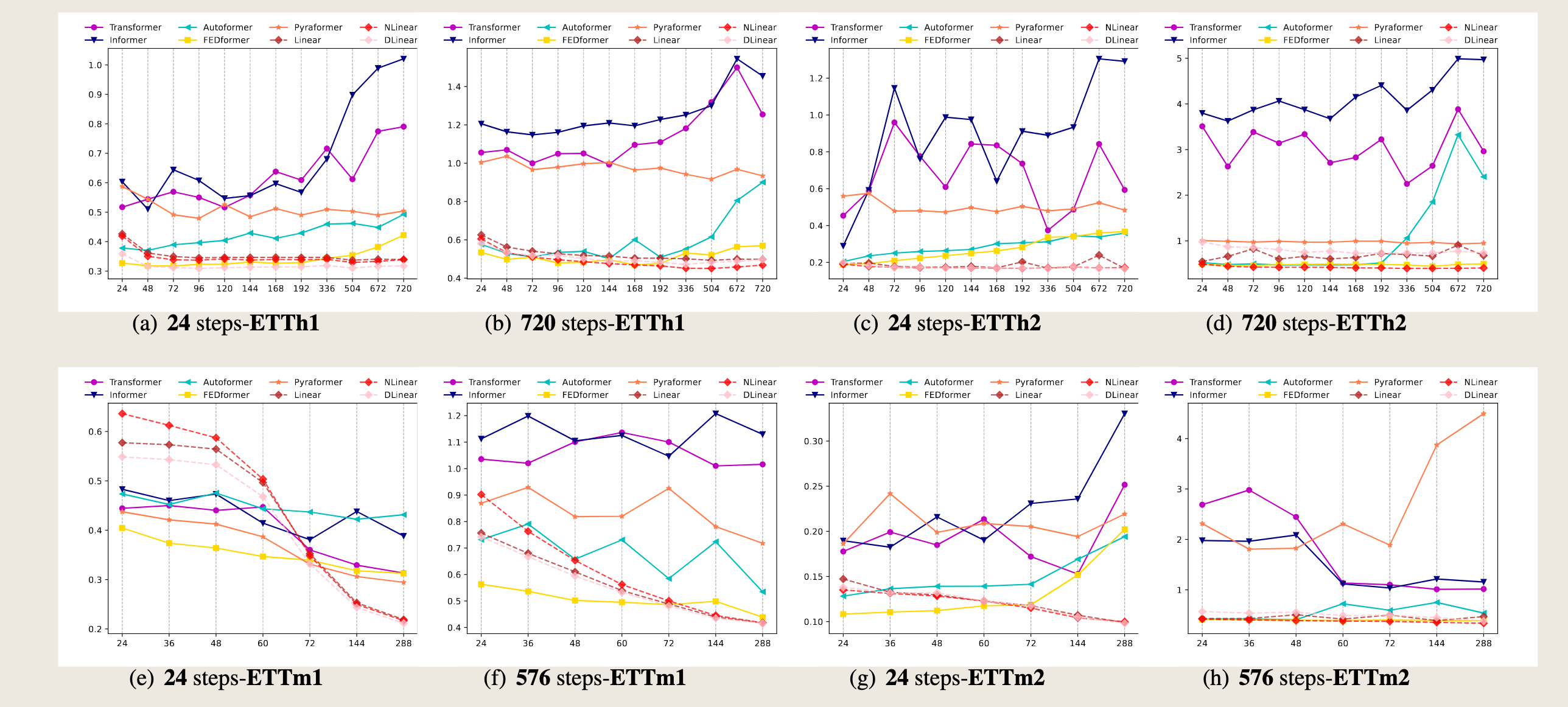
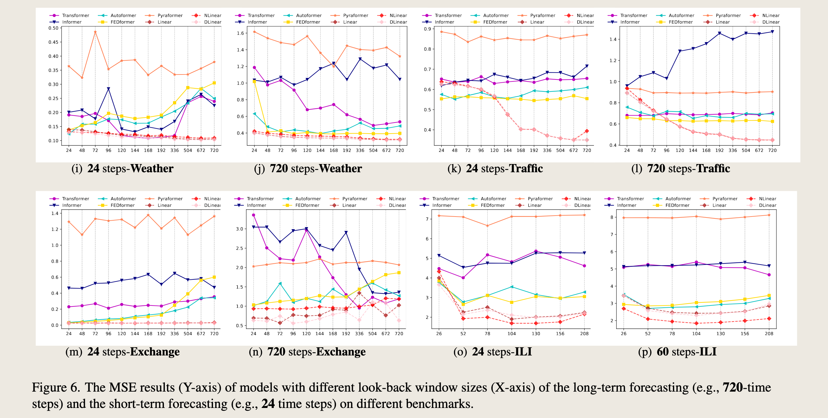
图6. 不同回溯窗口大小（X轴）下模型的均方误差（MSE）结果（Y轴），这些结果涵盖了长期预测（例如，720个时间步长）和短期预测（例如，24个时间步长）在不同基准测试上的表现。

D. Ablation study on the LTSF-Linear¶

D.1. Motivation of NLinear¶

If we normalize the test data by the mean and variance of train data, there could be a distribution shift in testing data, i.e, the mean value of testing data is not 0. If the model made a prediction that is out of the distribution of true value, a large error would occur. For example, there is a large error between the true value and the true value minus/add one.

如果我们根据训练数据的均值和方差对测试数据进行归一化，测试数据可能会出现分布偏移，即测试数据的均值不为0。如果模型做出的预测超出了真实值的分布范围，就会出现较大的误差。例如，真实值与真实值减一或加一之间存在较大的误差。

Therefore, in NLinear, we use the subtraction and addition to shift the model prediction toward the distribution of true value. Then, large errors are avoided, and the model performances can be improved. Figure 5 illustrates histograms of the trainset-test set distributions, where each bar represents the number of data points. Clear distribution shifts between training and testing data can be observed in ETTh1, ETTh2, and ILI. Accordingly, from Table 9 and Table 2 in the main paper, we can observe that there are great improvements in the three datasets comparing the NLinear to the Linear, showing the effectiveness of the NLinear in relieving distribution shifts. Moreover, for the datasets without obvious distribution shifts, like Electricity in Figure 5(c), using the vanilla Linear can be enough, demonstrating the similar performance with NLinear and DLinear.

因此，在NLinear中，我们使用减法和加法将模型预测向真实值的分布方向调整。这样，就可以避免大的误差，并且可以提高模型性能。图5展示了训练集-测试集分布的直方图，其中每个条形代表数据点的数量。在ETTh1、ETTh2和ILI中可以观察到训练数据和测试数据之间明显的分布偏移。相应地，从主论文中的表9和表2，我们可以观察到在这三个数据集上，将NLinear与Linear进行比较时，性能有显著提升，这显示了NLinear在缓解分布偏移方面的有效性。此外，对于没有明显分布偏移的数据集，如图5(c)中的电力数据集，使用传统的Linear可能就足够了，这表明Linear与NLinear和DLinear的性能相似。

D.2. The Features of LTSF-Linear¶

Although LTSF-Linear is simple, it has some compelling characteristics:

尽管LTSF-Linear模型简单，但它具有一些引人注目的特性：

An O(1) maximum signal traversing path length: The shorter the path, the better the dependencies are captured [18], making LTSF-Linear capable of capturing both short-range and long-range temporal relations.
$O(1)$的最大信号穿越路径长度：路径越短，捕获的依赖关系越好[18]，使得LTSF-Linear能够捕捉到短期和长期的时序关系。
High-efficiency: As LTSF-Linear is a linear model with two linear layers at most, it costs much lower memory and fewer parameters and has a faster inference speed than existing Transformers (see Table 8 in main paper).
高效率：由于LTSF-Linear最多包含两个线性层的线性模型，它的内存消耗更低，参数更少，并且比现有的Transformer具有更快的推理速度（见主论文中的表8）。
Interpretability: After training, we can visualize weights from the seasonality and trend branches to have some insights on the predicted values [9].
可解释性：训练后，我们可以从季节性和趋势分支中可视化权重，以对预测值有所了解[9]。
Easy-to-use: LTSF-Linear can be obtained easily without tuning model hyper-parameters.
易用性：LTSF-Linear可以轻松获得，无需调整模型超参数。

D.3. Interpretability of LTSF-Linear¶

Because LTSF-Linear is a set of linear models, the weights of linear layers can directly reveal how LTSFLinear works. The weight visualization of LTSF-Linear can also reveal certain characteristics in the data used for forecasting.

由于LTSF-Linear是一组线性模型，线性层的权重可以直接揭示LTSF-Linear的工作原理。LTSF-Linear的权重可视化还可以揭示用于预测的数据中的某些特征。

Here we take DLinear as an example. Accordingly, we visualize the trend and remainder weights of all datasets with a fixed input length of 96 and four different forecasting horizons. To obtain a smooth weight with a clear pattern in visualization, we initialize the weights of the linear layers in DLinear as 1/L rather than random initialization. That is, we use the same weight for every forecasting time step in the look-back window at the start of training.

这里我们以DLinear为例。相应地，我们可视化了所有数据集的趋势和残差权重，这些数据集具有固定的输入长度96和四个不同的预测范围。为了在可视化中获得平滑且具有清晰模式的权重，我们初始化DLinear中线性层的权重为$1/L$，而不是随机初始化。也就是说，在训练开始时，我们在回溯窗口中的每个预测时间步使用相同的权重。

**How the model works:**Figure 7(c) visualize the weights of the trend and the remaining layers on the Exchange-Rate dataset. Due to the lack of periodicity and seasonality in financial data, it is hard to observe clear patterns, but the trend layer reveals greater weights of information closer to the outputs, representing their larger contributions to the predicted values.

**模型工作原理：**图7(c)展示了汇率数据集上趋势层和剩余层的权重。由于金融数据缺乏周期性和季节性，很难观察到清晰的模式，但趋势层揭示了更接近输出的信息具有更大的权重，这代表了它们对预测值的更大贡献。

Periodicity of data: For Traffic data, as shown in Figure 7(d), the model gives high weights to the latest time step of the look-back window for the 0,23,47...719 forecast ing steps. Among these forecasting time steps, the 0, 167, 335, 503, 671 time steps have higher weights. Note that 24 time steps are a day, and 168 time steps are a week. This indicates that Traffic has a daily periodicity and a weekly periodicity.

数据的周期性：对于交通数据，如图7(d)所示，模型对于预测步长0、23、47...719的最新时间步赋予了较高的权重。在这些预测时间步中，0、167、335、503、671时间步的权重更高。请注意，24个时间步代表一天，168个时间步代表一周。这表明交通数据具有日周期性和周周期性。

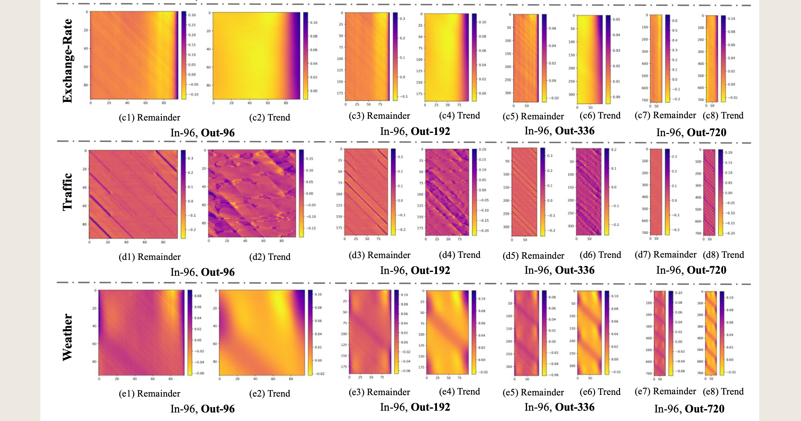
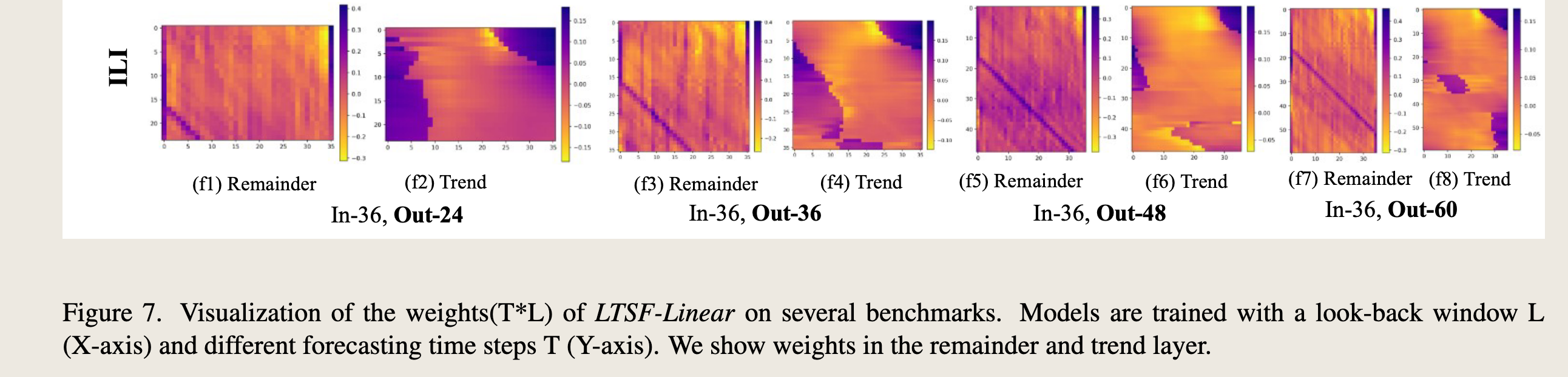
这幅图是LTSF-Linear模型在不同基准测试上的权重（T*L）可视化。图中展示了模型在回溯窗口大小为L（X轴）和不同的预测时间步长T（Y轴）下训练得到的权重。图中包括了趋势层（Trend）和残差层（Remainder）的权重。

具体来说，图中展示了以下四种情况的权重分布： 1. (f1) 和 (f3)：残差层的权重，分别对应预测步长为24和36。 2. (f2) 和 (f4)：趋势层的权重，分别对应预测步长为24和36。 3. (f5) 和 (f7)：残差层的权重，分别对应预测步长为48和60。 4. (f6) 和 (f8)：趋势层的权重，分别对应预测步长为48和60。

每个子图的X轴表示回溯窗口中的时间步长，Y轴表示预测的时间步长。颜色条表示权重的大小，颜色从蓝色（负权重）到黄色（正权重）变化，权重的绝对值越大，颜色越接近黄色。

通过这些可视化，可以观察到模型在不同时间步长上的权重分布情况，从而了解模型是如何从输入数据中学习时间依赖关系的。例如，可以观察到某些时间步长的权重在特定预测步长上更为显著，这可能表明这些时间步长对预测结果有更大的影响。

add_circle2025-03-01 21:43:55update2025-04-15 15:16:02