TDformer

• 题目:First De-Trend then Attend: Rethinking Attention for Time-Series Forecasting

• arxiv 日期: 2022 年 12 月15 日

• 期刊: NeurIPS2022 Workshop Attention

• 摘录本文重点: (We propose TDformer that separately models the trend with MLP and seasonality with Fourier attention)傅里叶变换频域注意力 建模季节性成分 ; 趋势性成分:MLP

• 划重点 ② we show that mathematically, time, Fourier and wavelet attention models are equivalent given linear assumptions.(线性注意力假设下的等价)

• 划重点③ Therefore, we find that frequency-domain attention models are capable of quickly recognizing the dominant frequency modes (more sample efficient) compared with time-domain models(因此，我们发现频率域注意力模型能够快速识别主导频率模式（更具样本效率），与时间域模型相比)

• 划重点④ linear attention still distributes attention to the noisy frequency modes, while softmax attention mostly focuses correctly on the dominant frequency modes. Therefore, frequency-domain attention models are more robust to spikes(频域注意力对噪声更加稳健)

• 附录对 季节性的度量进行的量化

Abstract

Transformer-based models have gained large popularity and demonstrated promising results in long-term time-series forecasting in recent years.

In addition to learning attention in time domain, recent works also explore learning attention in frequency domains (e.g., Fourier domain, wavelet domain), given that seasonal patterns can be better captured in these domains.

近年来，基于Transformer的模型在长期时间序列预测领域获得了广泛的关注，并取得了令人鼓舞的结果。除了在时间域学习注意力机制外，近期的研究还探索了在频率域（例如傅里叶域、小波域）中学习注意力机制，因为这些域能够更好地捕捉季节性模式。

In this work, we seek to understand the relationships between attention models in different time and frequency domains.

Theoretically, we show that attention models in different domains are equivalent under linear conditions (i.e., linear kernel to attention scores).

Empirically, we analyze how attention models of different domains show different behaviors through various synthetic experiments with seasonality, trend and noise, with emphasis on the role of softmax operation therein.

Both these theoretical and empirical analyses motivate us to propose a new method: TDformer (Trend Decomposition Transformer), that first applies seasonal-trend decomposition, and then additively combines an MLP which predicts the trend component with Fourier attention which predicts the seasonal component to obtain the final prediction.

Extensive experiments on benchmark time-series forecasting datasets demonstrate that TDformer achieves state-of-the-art performance against existing attention-based models.

在本工作中，我们试图理解不同时间域和频率域中注意力模型之间的关系。从理论上讲，我们证明了在满足线性条件（即注意力分数采用线性核）的情况下，不同域中的注意力模型是等价的。

通过各种包含季节性、趋势和噪声的合成实验，我们从经验上分析了不同域中的注意力模型表现出的不同行为，特别强调了softmax操作在此过程中的作用。

这些理论和经验分析激励我们提出了一种新方法：TDformer（趋势分解Transformer）。

该方法首先应用季节-趋势分解，然后将一个预测趋势分量的MLP（多层感知机）与预测季节性分量的傅里叶注意力机制相加性结合，以获得最终预测结果。

在基准时间序列预测数据集上的大量实验表明，TDformer在性能上达到了现有基于注意力机制的模型的最高水平。

Introduction

Transformer [1] recently gains wide popularity in time-series forecasting, inspired by its success in natural language processing and its ability to capture long-range dependencies [2]. Apart from the vanilla Transformer that calculates attention in time domain, recently variants of Transformer which calculate attention in frequency domains (e.g., Fourier domain or wavelet domain) (Figure 2) [3–7] have also been proposed to better model global characteristics of time series.

Transformer [1] 最近在时间序列预测领域获得了广泛的关注，这主要受到其在自然语言处理领域取得的成功以及其捕捉长距离依赖关系能力的启发 [2]。除了计算时间域注意力的标准Transformer（vanilla Transformer）之外，最近还提出了许多计算频率域（例如傅里叶域或小波域）注意力的Transformer变体（图2）[3–7]，以更好地建模时间序列的全局特征。

Despite the progress made by Transformer-based methods for time series forecasting, there lacks a rule of thumb to select the domain in which attention is best learned. Our work is driven by better understanding the following research question: Does learning attention in one domain offer better representation ability than the other? If so, how? We show mathematically that under linear conditions, learning attention in time or frequency domains leads to equivalent representation power. We then show that due to the softmax non-linearity used for normalization, this theoretical linear equivalence does not hold empirically. In particular, attention models in different domains demonstrate different empirical advantages. This finding sheds light on how to best apply attention models under different practical scenarios. We propose TDformer based on these insights and demonstrate that we achieve state-of-the-art performance against current attention-based models.

尽管基于Transformer的方法在时间序列预测方面取得了进展，但在选择最适合学习注意力的域方面，仍缺乏一个通用的规则。我们的研究动机在于更好地理解以下问题：在一个域中学习注意力是否比在另一个域中提供更好的表示能力？如果是，原因是什么？我们从数学上证明了在满足线性条件的情况下，无论在时间域还是频率域学习注意力，其表示能力是等价的。然而，由于用于归一化的softmax非线性操作，这种理论上的线性等价性在实际应用中并不成立。特别是，不同域中的注意力模型表现出不同的经验优势。这一发现为如何在不同的实际场景中最好地应用注意力模型提供了启示。基于这些见解，我们提出了TDformer，并证明了其在性能上达到了当前基于注意力模型的最高水平。

More specifically, we find that

(1) for data with strong seasonality, frequency-domain attention models are more sample-efficient compared with time-domain attention models, as softmax with exponential terms correctly amplify the dominant frequency modes in Fourier space.

（1）对于具有强季节性的数据，频率域注意力模型相比时间域注意力模型更加样本高效，因为softmax操作中的指数项能够正确地放大傅里叶空间中的主导频率模式。

(2) For data with trend, attention models generally show inferior generalizability, as attention models by nature interpolate rather than extrapolate the context. This finding of difference in performances of attention models on various types of time series data emphasizes the importance of seasonal-trend decomposition module in the attention model framework.

（2）对于具有趋势的数据，注意力模型通常表现出较差的泛化能力，因为注意力模型本质上是进行内插而不是外推上下文。

(3) For data with noisy spikes, frequency-domain attention models are more robust to such spiky data, as large-value spikes in the time domain correspond to small-amplitude high-frequency modes, whose attention would be filtered out by softmax operations.

（3）对于具有噪声尖峰的数据，频率域注意力模型对这种尖峰数据更具鲁棒性，因为时间域中的大值尖峰对应于小幅度的高频模式，这些模式的注意力会被softmax操作过滤掉。

Due to the different performances of the various attention modules on data with seasonality and trend, we propose TDformer that first decomposes the context time series into trend and seasonal components.

由于各种注意力模块在具有季节性和趋势的数据上表现不同，我们提出了TDformer，它首先将上下文时间序列分解为趋势和季节性成分。

We use a MLP for predicting the future trend, Fourier attention to predict the future seasonal part, and add these two components to obtain the final prediction.

我们使用MLP（多层感知机）来预测未来趋势，使用傅里叶注意力来预测未来的季节性部分，并将这两个成分相加以获得最终预测结果。

重点: MLP 预测趋势成分,傅里叶注意力预测季节成分

Extensive experiments on benchmark forecasting datasets demonstrate the effectiveness of our proposed approach. As a motivating example, we visualize predictions of TDformer and one of the best performing baselines FEDformer in Figure 1. On data with strong seasonality (Figure 1a and Figure 1b) TDformer preserves both the seasonality and trend of the original data, while FEDformer [5] deviates from the trend of the ground truth. On data with strong trend (Figure 1c and Figure 1d), TDformer generates predictions that better follow the trend of the original data.

在基准预测数据集上的大量实验验证了我们所提出方法的有效性。作为一个激励性示例，我们在图1中可视化了TDformer和表现最佳的基线模型之一FEDformer的预测结果。在具有强季节性的数据上（图1a和图1b），TDformer能够保留原始数据的季节性和趋势，而FEDformer [5]则偏离了真实值的趋势。在具有强趋势的数据上（图1c和图1d），TDformer生成的预测结果更能贴合原始数据的趋势。

本文贡献

In summary, our contributions are:

• We theoretically show that under linear conditions, attention models in time domain, Fourier domain and wavelet domain have the same representation power;
• 我们从理论上证明了在满足线性条件的情况下，时间域、傅里叶域和小波域中的注意力模型具有相同的表示能力
• We empirically analyze attention models in different domains with synthetic data of different characteristics, given the non-linearity of softmax. We show that frequency-domain attention performs the best on data with seasonality, and attention models in general have inferior generalizability on trend data, which motivates the design of a hybrid model based on seasonal trend decomposition;
• 我们通过具有不同特征的合成数据，对不同域中的注意力模型进行了经验分析，考虑到softmax的非线性特性。我们发现频率域注意力在具有季节性的数据上表现最佳，而注意力模型在趋势数据上通常泛化能力较差。这一发现促使我们基于季节-趋势分解设计了一种混合模型
• We propose TDformer that separately models the trend with MLP and seasonality with Fourier attention, and shows state-of-the-art performance against current attention models on time-series forecasting benchmarks.
• 我们提出了TDformer，它分别使用MLP建模趋势，使用傅里叶注意力建模季节性，并将这两个部分相加以获得最终预测结果。TDformer在时间序列预测基准测试中达到了当前注意力模型的最高水平

本文重点: 傅里叶变换频域注意力 建模季节性成分 ; 趋势性成分:MLP

Related Work

分成频域模型和时域模型叙述的

实际上应该是:

RNN 系,former 系,Linear 系

单输入,多输入

短时预测,长时预测

Time-Domain Attention Forecasting Models. Informer [3] proposes efficient ProbSparse selfattention mechanism. Autoformer [4] renovates time-series decomposition as a basic inner block and designs Auto-Correlation mechanism for dependencies discovery. Non-stationary Transformer [7] proposes Series Stationarization and De-stationary Attention to address over-stationarization.

时间域注意力预测模型。Informer [3] 提出了高效的ProbSparse自注意力机制。Autoformer [4] 将时间序列分解作为基础内部模块进行革新，并设计了自相关机制以发现依赖关系。非平稳Transformer [7] 提出了序列平稳化和去平稳化注意力机制，以解决过度平稳化的问题。

时域模型

• Informer
• Autoformer
• Non-stationary Transformer

Frequency-Domain Attention Forecasting Models.

FEDformer [5] proposes Fourier and wavelet enhanced blocks based on Multiwavelet-based Neural Operator Learning [8] to capture important structures in time series through frequency domain mapping.

频率域注意力预测模型。FEDformer [5] 基于多小波神经算子学习 [8] 提出了傅里叶和小波增强模块，通过频率域映射捕捉时间序列中的重要结构。

ETSformer [6] selects top-K largest amplitude modes as frequency attention and combines with exponential smoothing attention.

ETSformer [6] 选择振幅最大的前K个模式作为频率注意力，并结合指数平滑注意力。

Adaptive Fourier Neural Operator (AFNO) [9] builds upon FNO [10] and proposes an efficient token mixer that learns to mix in the Fourier domain.

自适应傅里叶神经算子（AFNO）[9] 基于FNO [10] 提出了一种高效的标记混合器，用于在傅里叶域中学习混合。

FNet [11] replaces the self-attention with Fourier Transform and promotes efficiency without much loss of accuracy on NLP benchmarks.

FNet [11] 用傅里叶变换替换了自注意力机制，在自然语言处理基准测试中提高了效率且几乎没有损失准确性。

T-WaveNet [12] constructs a tree-structured network with each node built with invertible neural network (INN) based wavelet transform unit for iterative decomposition.

T-WaveNet [12] 构建了一个树形结构网络，每个节点都基于可逆神经网络（INN）的小波变换单元进行迭代分解。

Adaptive Wavelet Transformer Network (AWT-Net) [13] generates wavelet coefficients to classify each point into high or low sub-bands components and exploits Transformer to enhance the original shape features.

自适应小波Transformer网络（AWT-Net）[13] 生成小波系数，将每个点分类为高频或低频子带分量，并利用Transformer增强原始形状特征。

频域模型

• FEDformer
• ETSformer
• Adaptive Fourier Neural Operator (AFNO)
• FNet
• T-WaveNet
• Adaptive Wavelet Transformer Network (AWT-Net)

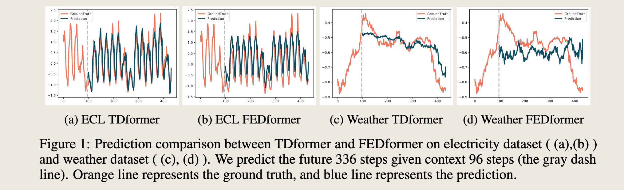
比较预测结果,输入 96 时间步,输出 336 时间步

灰色线,后开始是 yuce,橙色线是真实值,蓝色线是预测值

时域注意力,频域注意力,小波注意力比较

Decomposition-Based Forecasting Models decompose time series into trend and seasonality (with i.e., STL decomposition [14]). Apart from attention-based Autoformer and FEDformer, N-BEATS [15] models trend with small-degree polynomials and seasonality with Fourier series. N-HiTS [16] redefines N-BEATS by enhancing its input decomposition via multi-rate data sampling and its output synthesizer via multi-scale interpolation. FreDo [17] incorporates frequency-domain features into AverageTile model that averages history sub-series. FiLM [18] applies Legendre Polynomials projections to approximate historical information and Fourier projection to remove noise. DeepFS [19] encodes temporal patterns with self-attention and predicts Fourier series parameters and trend with MLP.

基于分解的时间序列预测模型将时间序列分解为趋势和季节性成分（例如，使用STL分解 [14]）。除了基于注意力机制的Autoformer和FEDformer之外，N-BEATS [15] 使用低阶多项式建模趋势，使用傅里叶级数建模季节性。N-HiTS [16] 通过多速率数据采样增强其输入分解，通过多尺度插值增强其输出合成器，从而重新定义了N-BEATS。FreDo [17] 将频率域特征整合到AverageTile模型中，该模型通过平均历史子序列来预测。FiLM [18] 应用勒让德多项式投影来近似历史信息，并使用傅里叶投影去除噪声。DeepFS [19] 使用自注意力对时间模式进行编码，并通过MLP预测傅里叶级数参数和趋势。

基于分解的预测模型

这里的相关工作介绍的内容

• 时域方法
• 频域方法
• 基于分解的预测

Despite the success of attention models in time, Fourier, and wavelet domains, there is still a lack of notion for understanding their relationships and respective advantages. Decomposition-based methods also adopt decomposition layers without giving strong reasoning for their necessity. We propose to fill this gap from both theoretical and empirical perspectives, and based on these analysis build a new framework that shows better forecasting performance.

尽管注意力模型在时间域、傅里叶域和小波域都取得了成功，但目前仍然缺乏对它们之间关系以及各自优势的理解。基于分解的方法虽然采用了分解层，但并没有给出其必要性的有力理由。我们提出从理论和经验两个角度来填补这一空白，并基于这些分析构建一个新的框架，以展示更好的预测性能。

本文的动机,分解为什么有用,以及什么时候用分解

Linear Equivalence of Attention in Various Domains

Formulation of Attention Models

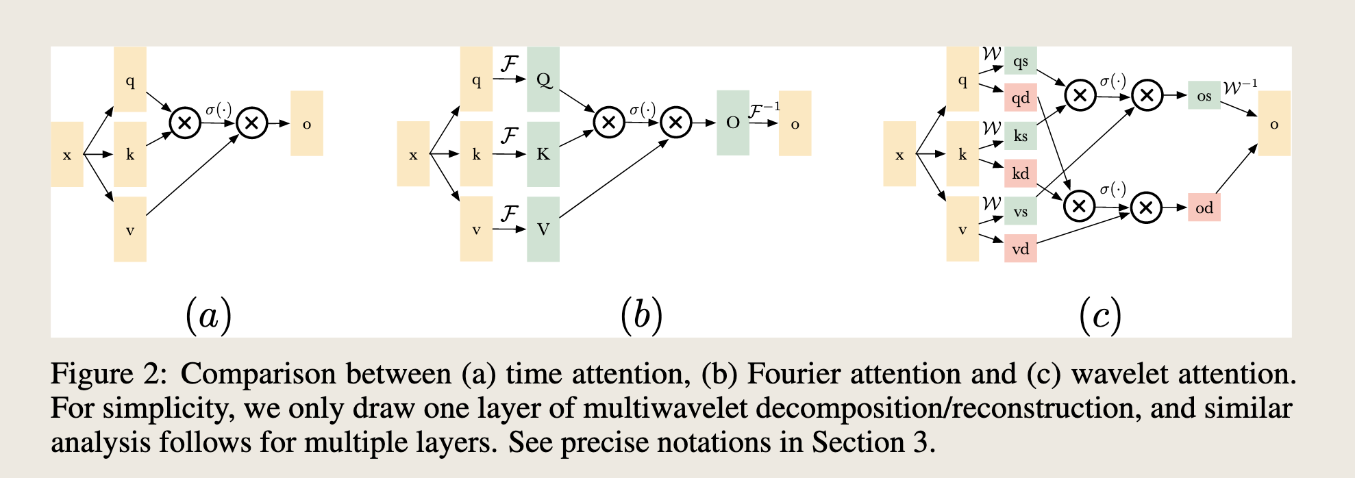
We first briefly introduce the canonical Transformers. Denote input queries, keys and values as $q \in \mathbb{R}^{L \times D}, k \in \mathbb{R}^{L \times D}, v \in \mathbb{R}^{L \times D}$, which are transformed from input $x$ through linear embeddings. Denote output of attention module as $o(q, k, v) \in \mathbb{R}^{L \times D}$. As shown in Figure 2 (a), The attention operation in canonical attention is formulated as

where $d_q$ is the dimension for queries that serves as normalization term in attention operation, and $\sigma(\cdot)$ represents activation function. When $\sigma(\cdot) = \text{softmax}(\cdot)^3$, we have softmax attention: $o(q, k, v) = \text{softmax} \left( \frac{q k^T}{\sqrt{d_q}} \right) v$. When $\sigma(\cdot) = \text{Id}(\cdot)$ (identity mapping), we have linear attention: $o(q, k, v) = q k^T v$ (we ignore the normalization term $\sqrt{d_q}$ for simplicity).

我们首先简要介绍标准的Transformer模型。将输入的查询（queries）、键（keys）和值（values）表示为 $q \in \mathbb{R}^{L \times D}, k \in \mathbb{R}^{L \times D}, v \in \mathbb{R}^{L \times D}$，这些是通过输入 $x$ 经过线性嵌入转换得到的。将注意力模块的输出表示为 $o(q, k, v) \in \mathbb{R}^{L \times D}$。如图2(a)所示，标准注意力中的注意力操作被定义为

其中 $d_q$ 是查询的维度，它在注意力操作中作为归一化项，$\sigma(\cdot)$ 表示激活函数。当 $\sigma(\cdot) = \text{softmax}(\cdot)^3$ 时，我们得到softmax注意力：$o(q, k, v) = \text{softmax} \left( \frac{q k^T}{\sqrt{d_q}} \right) v$。当 $\sigma(\cdot) = \text{Id}(\cdot)$（恒等映射）时，我们得到线性注意力：$o(q, k, v) = q k^T v$（为了简化，我们忽略了归一化项 $\sqrt{d_q}$）。

Definition 3.1 (Time Attention). Equation 1 refers to time domain attention where q, k, v are all in original time domain, shown in Figure 2 (a).

定义 3.1（时间域注意力）。方程 1 指的是时间域注意力，其中 $q$，$k$，$v$ 都在原始时间域中，如图 2 (a) 所示。

Definition 3.2 (Fourier Attention). Fourier attention first converts queries, keys, and values with Fourier Transform, performs a similar attention mechanism in the frequency domain, and finally converts the results back to the time domain using inverse Fourier transform, shown in Figure 2 (b). Let $\mathcal{F}(\cdot), \mathcal{F}^{-1}(\cdot)$ denote Fourier transform and inverse Fourier transform, then Fourier attention is $o(q, k, v) = \mathcal{F}^{-1} \left( \sigma \left( \mathcal{F}(q) \overline{\mathcal{F}(k)}^T / \sqrt{d_q} \right) \mathcal{F}(v) \right)$.

定义 3.2（傅里叶注意力）。傅里叶注意力首先使用傅里叶变换将查询（queries）、键（keys）和值（values）转换到频率域，执行与时间域相似的注意力机制，最后使用逆傅里叶变换将结果转换回时间域，如图 2 (b) 所示。设 $\mathcal{F}(\cdot), \mathcal{F}^{-1}(\cdot)$ 表示傅里叶变换和逆傅里叶变换，则傅里叶注意力为 $o(q, k, v) = \mathcal{F}^{-1} \left( \sigma \left( \mathcal{F}(q) \overline{\mathcal{F}(k)}^T / \sqrt{d_q} \right) \mathcal{F}(v) \right)$。

Definition 3.3 (Wavelet Attention). Wavelet transform applies wavelet decomposition and reconstruction to obtain signals of different scales. Wavelet attention performs attention calculation to decomposed queries, keys, and values in each scale, and reconstructs the output from attention results in each scale, illustrated in Figure 2 (c). Let $\mathcal{W}(\cdot), \mathcal{W}^{-1}(\cdot)$ denote wavelet decomposition and wavelet reconstruction, then wavelet attention is $o(q, k, v) = \mathcal{W}^{-1} \left( \sigma \left( \mathcal{W}(q) \mathcal{W}(k)^T / \sqrt{d_q} \right) \mathcal{W}(v) \right)$.

定义 3.3（小波注意力）。小波变换应用小波分解和重构来获取不同尺度的信号。小波注意力对每个尺度中分解后的查询（queries）、键（keys）和值（values）执行注意力计算，并从小波注意力结果中重构输出，如图 2 (c) 所示。设 $\mathcal{W}(\cdot), \mathcal{W}^{-1}(\cdot)$ 表示小波分解和小波重构，则小波注意力为 $o(q, k, v) = \mathcal{W}^{-1} \left( \sigma \left( \mathcal{W}(q) \mathcal{W}(k)^T / \sqrt{d_q} \right) \mathcal{W}(v) \right)$。

Linear Equivalence of Time, Fourier and Wavelet Attention

In this section we formally prove that time, Fourier and wavelet attention models are equivalent under linear attention case.

在本节中，我们正式证明时间域、傅里叶域和小波域注意力模型在线性注意力情况下是等价的。

Lemma 3.1. When $\sigma(\cdot) = \text{Id}(\cdot)$ (linear attention), time, Fourier and wavelet attention are equivalent.

引理 3.1：当 $\sigma(\cdot) = \text{Id}(\cdot)$（线性注意力）时，时间域、傅里叶域和小波域注意力是等价的。

Proof. Let $\mathbf{W} = \left( \frac{\omega^{jk}}{\sqrt{L}} \right) \in \mathbb{C}^{L \times L}, \omega = e^{-\frac{2\pi j}{L}}$ denote the Fourier matrix, then Fourier transform to signal $x \in \mathbb{R}^{L \times D}$ can be expressed as $\mathbf{X} = \mathbf{W}x, \mathbf{X} \in \mathbb{C}^{L \times D}$, and inverse Fourier transform can be expressed as $x = \mathbf{W}^H \mathbf{X}$, where $\mathbf{W}^H$ is the Hermitian (conjugate transpose) of $\mathbf{W}$. Given properties of Fourier matrix, we could easily show that

Following this expression, Fourier domain linear attention can be written as

证明：设 $\mathbf{W} = \left( \frac{\omega^{jk}}{\sqrt{L}} \right) \in \mathbb{C}^{L \times L}, \omega = e^{-\frac{2\pi j}{L}}$ 表示傅里叶矩阵，则信号 $x \in \mathbb{R}^{L \times D}$ 的傅里叶变换可以表示为 $\mathbf{X} = \mathbf{W}x, \mathbf{X} \in \mathbb{C}^{L \times D}$，逆傅里叶变换可以表示为 $x = \mathbf{W}^H \mathbf{X}$，其中 $\mathbf{W}^H$ 是 $\mathbf{W}$ 的厄米共轭（共轭转置）。根据傅里叶矩阵的性质，我们可以轻松证明

根据这个表达式，傅里叶域的线性注意力可以写为

Therefore, calculating attention in Fourier domain is equivalent to time-domain attention.

因此，在傅里叶域中计算注意力等同于在时间域中计算注意力。

For wavelet attention, we take single-scale wavelet decomposition and reconstruction as an example, and multi-scale wavelet transform follows the same analysis.

对于小波注意力，我们以单尺度小波分解和重构为例，多尺度小波变换遵循相同的分析。

Using the same notation, let $\mathbf{W} \in \mathbb{R}^{L \times \frac{L}{2}}, \mathbf{W}^{-1} \in \mathbb{R}^{\frac{L}{2} \times L}$ denote the wavelet decomposition and reconstruction matrix, then wavelet decomposition to signal $x \in \mathbb{R}^{L \times D}$ can be expressed as $\mathbf{X} = \mathbf{W}x, \mathbf{X} \in \mathbb{R}^{\frac{L}{2} \times D}$, and wavelet reconstruction can be expressed as $x = \mathbf{W}^{-1}\mathbf{X}$. Since wavelet matrix is orthogonal, we have the property that $\mathbf{W}^T\mathbf{W} = \mathbf{I}$. Wavelet linear attention is

which is again equivalent to time-domain attention. Therefore, we show that mathematically, time, Fourier and wavelet attention models are equivalent given linear assumptions.

使用相同的符号，设 $\mathbf{W} \in \mathbb{R}^{L \times \frac{L}{2}}, \mathbf{W}^{-1} \in \mathbb{R}^{\frac{L}{2} \times L}$ 表示小波分解和重构矩阵，那么信号 $x \in \mathbb{R}^{L \times D}$ 的小波分解可以表示为 $\mathbf{X} = \mathbf{W}x, \mathbf{X} \in \mathbb{R}^{\frac{L}{2} \times D}$，小波重构可以表示为 $x = \mathbf{W}^{-1}\mathbf{X}$。由于小波矩阵是正交的，我们有性质 $\mathbf{W}^T\mathbf{W} = \mathbf{I}$。小波线性注意力为

这同样等同于时间域注意力。因此，我们数学上证明了，在给定线性假设的情况下，时间域、傅里叶域和小波域注意力模型是等价的。

结论:在线性注意力的条件下, 时域,傅里叶,小波域是等价的

Investigation on the Role of Softmax

这部分讨论 softmax 的角色

Although these attention models are equivalent given linear assumptions, in practice we apply softmax as normalization, which changes the behavior of different attention models. In this section, we empirically analyze how softmax causes such performance gaps on datasets with three different representative properties: seasonality, trend and noise. For all experiments in this section, the task is to predict the next 96 time steps given history 96 time steps. We implement the wavelet-domain attention model based on multiwavelet transform model [8].

尽管在给定线性假设的情况下这些注意力模型是等价的，但在实践中我们应用softmax作为归一化，这改变了不同注意力模型的行为。在本节中，我们通过实验分析了softmax如何在具有三种不同代表性特征的数据集上导致性能差距：季节性、趋势和噪声。在本节的所有实验中，任务是基于历史96个时间步长来预测接下来的96个时间步长。我们基于多小波变换模型[8]实现了小波域注意力模型。

Data with Seasonality

For data with fixed seasonality, Fourier attention is the most sample-efficient. We use sin(x) as an example of seasonal data (visualized in Figure 3a and Figure 3b). There exist dominant frequency modes for data with seasonality. We visualize linear attention (Figure 3c) and softmax attention (Figure 3d) in Fourier space. Attention scores are concentrated on the dominant frequency mode. As softmax with exponential terms has the “polarization” effect (increasing the gap between large and small values), softmax attention further concentrates the scores on the dominant frequency, helping the model to better capture seasonal information. Therefore, we find that frequency-domain attention models are capable of quickly recognizing the dominant frequency modes (more sample efficient) compared with time-domain models (Figure 4a).

对于具有固定季节性的数据，傅里叶注意力是最具有样本效率的。我们使用 $\sin(x)$ 作为季节性数据的例子（在图3a和图3b中可视化）。对于具有季节性的数据，存在主导的频率模式。我们在傅里叶空间中可视化线性注意力（图3c）和softmax注意力（图3d）。注意力分数集中在主导频率模式上。由于具有指数项的softmax具有“极化”效应（增加大值和小值之间的差距），softmax注意力进一步将分数集中在主导频率上，帮助模型更好地捕捉季节性信息。因此，我们发现频率域注意力模型能够快速识别主导频率模式（更具样本效率），与时间域模型相比（图4a）。

softmax 的极化效应

图三的描述: Figure 3: (a)-(d): Data with fixed seasonality: sin(x). Fourier softmax attention amplifies the correct frequency modes compared with Fourier linear attention.

图3：(a)-(d)：具有固定季节性的数据：$\sin(x)$。傅里叶softmax注意力与傅里叶线性注意力相比，放大了正确的频率模式。

(e)-(h): Data with varying seasonality. Fourier softmax attention amplifies the dominant frequency modes, but also neglects the small amplitude modes that embed the localized frequency information.

(e)-(h)：具有变化季节性的数据。傅里叶softmax注意力放大了主导频率模式，但也忽略了嵌入局部化频率信息的小幅度模式。

(i)-(l): Data with linear trend. Fourier softmax attention incorrectly amplifies the low-frequency modes compared with Fourier linear attention.

(i)-(l)：具有线性趋势的数据。傅里叶softmax注意力与傅里叶线性注意力相比，错误地放大了低频模式。

(m)-(p): Data with spikes as noise. Fourier softmax attention filters out the noisy components and emphasizes the correct frequency modes compared with Fourier linear attention.

(m)-(p)：具有尖峰噪声的数据。傅里叶softmax注意力与傅里叶线性注意力相比，滤除了噪声成分，并强调了正确的频率模式。

To further illustrate such polarization effect, we also compare softmax attention with polynomial kernels $\sigma(x) = x_i^d / \sum_i x_i^d$, where $d$ is the degree of polynomials (without loss of generality we assume $x_i > 0, \forall i$). Polarization effect increases with respect to polynomial degrees. As shown in Figure 4c, the performance also increases as we increase the polarization effect and approaches the performance of softmax operations. We also notice that apart from the polarization effect from exponential terms, normalization itself also introduces performance gaps between different attention models. The possible reason is that it’s easier to optimize in the sparse Fourier domain compared with time domain. We leave this as our future explorations.

为了进一步说明这种极化效应，我们还比较了softmax注意力与多项式核 $\sigma(x) = x_i^d / \sum_i x_i^d$，其中 $d$ 是多项式的度数（不失一般性，我们假设 $x_i > 0, \forall i$）。极化效应随着多项式度数的增加而增加。如图4c所示，随着极化效应的增加，性能也随之提高，并接近softmax操作的性能。我们还注意到，除了来自指数项的极化效应外，归一化本身也在不同的注意力模型之间引入了性能差距。可能的原因是，在稀疏的傅里叶域中优化比在时间域中更容易。我们将此作为未来的探索方向。

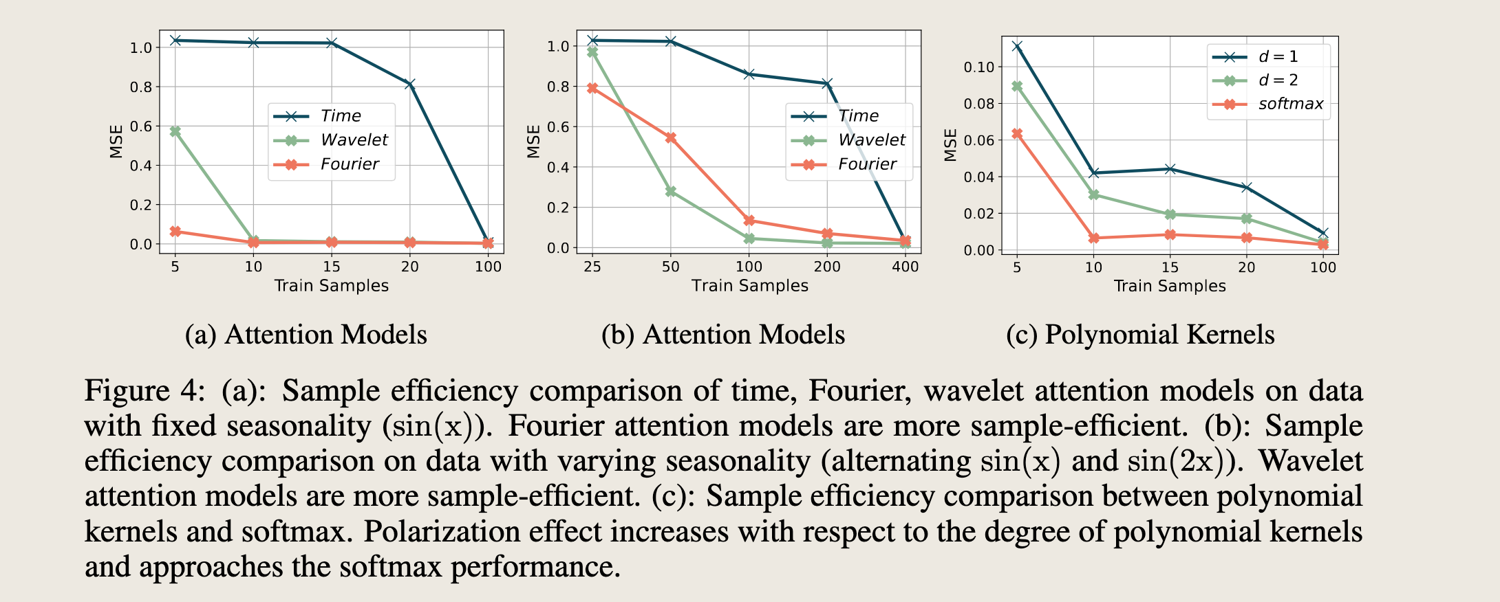
图4：（a）：在具有固定季节性（$\sin(x)$）的数据上，时间域、傅里叶域和小波域注意力模型的样本效率比较。傅里叶注意力模型具有更高的样本效率。（b）：在季节性变化的数据上（交替的$\sin(x)$和$\sin(2x)$）的样本效率比较。小波注意力模型具有更高的样本效率。（c）：多项式核与softmax之间的样本效率比较。随着多项式核度数的增加，极化效应增加，并接近softmax性能。

For data with varying seasonality, wavelet attention is the most effective. We use alternating $\sin(x)$ and $\sin(2x)$ as an example of varying seasonal data (visualized in Figure 3e and Figure 3f). The Fourier representation has both dominant modes as well as small-amplitude modes, where the latter embeds the varying-seasonality information. The Fourier softmax attention correctly amplifies the dominant frequency modes, but at the same time neglects the small-amplitude modes that convey the information of varying seasonality. By contrast, wavelet attention combines multi-scale time-frequency representation, and provides better localized frequency information. As shown in Figure 4b, wavelet attention is the most effective for varying-seasonality data.

对于具有变化季节性的数据，小波注意力模型最为有效。我们使用交替的 $\sin(x)$ 和 $\sin(2x)$ 作为变化季节性数据的例子（在图3e和图3f中可视化）。傅里叶表示既包含主导模式也包含小幅度模式，后者嵌入了变化的季节性信息。傅里叶softmax注意力正确地放大了主导频率模式，但同时忽略了传递变化季节性信息的小幅度模式。相比之下，小波注意力结合了多尺度时频表示，并提供了更好的局部化频率信息。如图4b所示，小波注意力对于变化季节性数据最为有效。

Data with Trend

For data with trend, all attention models show inferior generalizability, especially Fourier attention. We take linear trend data as an example (Figure 3i and Figure 3j) and evaluate different attention models. The first several frequency modes in Fourier space carry large values; the attention scores hence mostly focus on the first few frequency modes (top-left corner of Figure 3k). With the polarization effect of softmax, attention scores emphasize even more on these low-frequency components (Figure 3l) and generate misleading reconstruction results. We evaluate different attention models in Table 1. Fourier attention, with inappropriate polarization, leads to the largest errors.

对于具有趋势的数据，所有注意力模型都显示出较差的泛化能力，尤其是傅里叶注意力。我们以线性趋势数据为例（图3i和图3j），并评估不同的注意力模型。傅里叶空间中的前几个频率模式具有较大的值；因此，注意力分数主要集中于最初的几个频率模式（图3k的左上角）。由于softmax的极化效应，注意力分数更加强调这些低频分量（图3l），并产生了误导性的重构结果。我们在表1中评估了不同的注意力模型。傅里叶注意力由于极化不当，导致了最大的误差。

Moreover, all these attention models fail to extrapolate linear trend well and suffer from large errors, since attention mechanism by nature works through interpolating the context history. By contrast, MLP perfectly predicts such trend signals, as shown in Table 1. This motivates us to decompose the time series into trend and seasonality [4, 5], apply attention mechanism only for seasonality, and use MLP for modeling trend.

此外，所有这些注意力模型都无法很好地外推线性趋势，并因误差较大而受到影响，因为注意力机制本质上是通过插值上下文历史来工作的。相比之下，如图1所示，多层感知机（MLP）能够完美预测此类趋势信号。这激励我们将时间序列分解为趋势和季节性[4, 5]，仅对季节性应用注意力机制，并使用MLP来建模趋势。

Data with Spikes

Data with Spikes 含有尖峰的数据

For data carrying noise, Fourier attention is the most robust. We randomly inject large-value spikes into the training set of $\sin(x)$ as a motivating example (Figure 3m and Figure 3n). Spikes which have large values in time domain result in small-amplitude frequency components after Fourier transforms. With the polarization effect of softmax, time-domain softmax attention focuses incorrectly on large-value spikes while Fourier-domain softmax attention correctly filters out the noisy components and attends to the dominant frequency modes induced by $\sin(x)$. Comparing Figure 3o and Figure 3p, linear attention still distributes attention to the noisy frequency modes, while softmax attention mostly focuses correctly on the dominant frequency modes. Therefore, frequency-domain attention models are more robust to spikes, as shown in Table 2. All these analysis on datasets with different characteristics help guide our model design in the next section.

对于携带噪声的数据，傅里叶注意力最为稳健。我们随机将大值尖峰注入到 $\sin(x)$ 的训练集中作为一个激励性示例（图3m和图3n）。在时间域中具有大值的尖峰在经过傅里叶变换后会产生小幅度的频率分量。由于softmax的极化效应，时间域softmax注意力错误地集中在大值尖峰上，而傅里叶域softmax注意力正确地滤除了噪声成分，并关注由 $\sin(x)$ 引起的主导频率模式。比较图3o和图3p，线性注意力仍然将注意力分配给噪声频率模式，而softmax注意力大多正确地集中在主导频率模式上。因此，频率域注意力模型对尖峰更为稳健，如表2所示。所有这些针对具有不同特征的数据集的分析有助于指导我们在下一节中的模型设计。

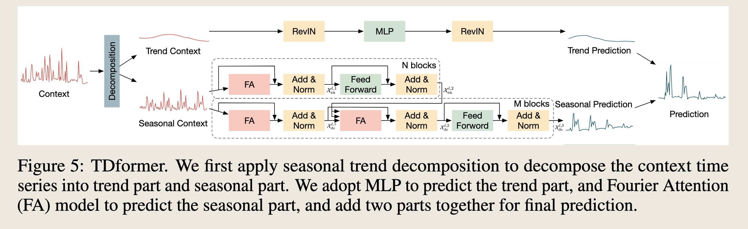
TDformer。我们首先应用季节-趋势分解将上下文时间序列分解为趋势部分和季节性部分。我们采用多层感知机（MLP）来预测趋势部分，并使用傅里叶注意力（FA）模型来预测季节性部分，然后将这两部分相加以获得最终预测。

Our Method: TDformer

The performance difference in data with various characteristics motivates our model design. For data with seasonality, Fourier softmax attention amplifies dominant frequency modes and demonstrates the best performance. For data with trend, Fourier softmax incorrectly attends to only the low-frequency modes and produces large errors. Meanwhile, all attention models which work through interpolating the historical context, do not generalize well on trend data compared with MLP. These analyses motivate us to decompose time series into trend and seasonality, use Fourier attention to predict the seasonal part and MLP to predict the trend part. Figure 5 overviews our proposed model architecture.

不同特征数据中的性能差异激发了我们的模型设计。对于具有季节性的数据，傅里叶softmax注意力放大了主导频率模式，并展现出最佳性能。对于具有趋势的数据，傅里叶softmax错误地仅关注低频模式并产生较大误差。同时，所有通过插值历史上下文工作的注意力模型在趋势数据上的泛化能力不如多层感知机（MLP）。这些分析促使我们将时间序列分解为趋势和季节性，使用傅里叶注意力来预测季节性部分，使用MLP来预测趋势部分。图5概述了我们提出的模型架构。

这段在总结,傅里叶哪里好,模型的设计理由分析傅里叶的优劣

讨论的对象是:

• 模型层面: MLP & 傅里叶 softmax 注意力
• 数据层面: 趋势性成分 & 季节性成分

第一步:(分解)

We first decompose the time series into trend parts and seasonal parts following FEDformer [5]. More specifically, we apply multiple average filters with different sizes to extract different trend patterns, and apply adaptive weights to combine these patterns into the final trend component. The seasonal component is acquired by subtracting trend from the original time series:

我们首先按照FEDformer[5]的方法将时间序列分解为趋势部分和季节性部分。更具体地说，我们应用多个不同尺寸的平均滤波器来提取不同的趋势模式，并应用自适应权重将这些模式组合成最终的趋势成分。季节性成分是通过从原始时间序列中减去趋势得到的：

$\mathrm{x_{trend}=\sigma(\omega(x))*f(x),x_{seasonal}=x-x_{trend}}$

值得注意的是:

①参考了 FEDFormer的分解方法,分解为季节项&趋势项

②注意:设计多个不同尺寸的平均滤波器提取趋势成分

符号说明:

where $σ, w(x), f (x)$ denote the softmax operation, data-dependent weights and average filters.

• $\sigma$ softmax
• $\omega(x)$ 数据依赖的权重
• f(x) 是平均滤波器

第二步( 对于趋势性成分的处理)

For the trend component, we use a three-layer MLP to predict the future trend. As reversible instance normalization (RevIN) proves to be effective to remove and restore the non-stationary information [20, 18] which mainly resides in trend, we also add RevIN layers before and after MLP:

对于趋势成分，我们使用三层MLP来预测未来的趋势。由于可逆实例归一化（RevIN）被证明对于移除和恢复主要存在于趋势中的非平稳信息是有效的[20, 18]，我们还在MLP前后添加了RevIN层：

第三步(对于季节性成分处理)

For the seasonal component, we adopt Transformer architecture but replace time-domain attention with Fourier-domain attention. More specifically, we first feed the seasonal part to $N$ layers of encoder:

where $\mathcal{X}_{\text{en}}^0 = \mathbf{x}_{\text{seasonal}}$, FA and FF are short for Fourier Attention and Feed Forward network.

对于季节性成分，我们采用Transformer架构，但将时域注意力替换为傅里叶域注意力。更具体地说，我们首先将季节性部分输入到$N$层编码器中：

其中 $\mathcal{X}_{\text{en}}^0 = \mathbf{x}_{\text{seasonal}}$，FA和FF分别是傅里叶注意力和前馈网络的缩写。

傅里叶计算的过程

Fourier Attention computes the attention in Fourier space and converts the output to time domain at the end (Definition 3.2) with $\sigma(\cdot) = \text{softmax}(\cdot)$:

The seasonal part is also zero-padded for the future part and fed into $M$ layers of decoder to obtain the final seasonal output:

where $\mathcal{X}_{\text{de}}^0 = \text{Padding}(\mathbf{x}_{\text{seasonal}})$.

We add the trend prediction from MLP and seasonal prediction from Transformer to obtain the final output prediction, i.e.,

$\mathcal{X}_{\text{final}} = \mathcal{X}_{\text{trend}} + \mathcal{X}^M_{\text{de}}$.

Optimization is based on a reconstruction MSE loss between predicted and ground truth future time series.

傅里叶注意力在傅里叶空间计算注意力，最后将输出转换到时域（定义3.2），其中 $\sigma(\cdot) = \text{softmax}(\cdot)$：

季节性部分也为未来部分进行了零填充，并输入到$M$层解码器中以获得最终的季节性输出：

其中 $\mathcal{X}^0_{\text{de}} = \text{Padding}(\mathbf{x}_{\text{seasonal}})$ 。

我们将MLP的趋势预测和Transformer的季节性预测相加，以获得最终的输出预测，即 $\mathcal{X}_{\text{final}} = \mathcal{X}_{\text{trend}} + \mathcal{X}^M_{\text{de}}$。优化基于预测和真实未来时间序列之间的重构均方误差（MSE）损失。

Remark. While FEDformer [5] and Autoformer [4] also have seasonal-trend decomposition, their trend and seasonal components are not disentangled; the trend prediction still comes from the attention module, which is sub-optimal based on our analysis in Section 4 and our empirical results in Section 6. By contrast, we apply seasonal-trend decomposition in the beginning, and apply Fourier attention only on seasonality components. This seemingly simple different way of decomposition brings significant performance gains to see in the experiment section, with even less model complexity. Non-stationary Transformer also computes attention for trend data. Moreover, with RevIN, TDformer has the similar effect of stationarization.

备注。 尽管FEDformer[5]和Autoformer[4]也进行了季节-趋势分解，但他们的趋势和季节成分并没有完全分离；趋势预测仍然来自注意力模块，这根据我们在第4节的分析和第6节的实验结果来看是次优的。相比之下，我们在开始时就应用季节-趋势分解，并仅对季节性成分应用傅里叶注意力。这种看似简单的不同分解方式在实验部分带来了显著的性能提升，并且模型复杂度更低。非平稳Transformer也对趋势数据计算注意力。此外，通过使用RevIN，TDformer具有类似的平稳化效果。

Experiments

Dataset and Baselines

We conduct experiments on benchmark time-series forecasting datasets: ETTm2 [3], electricity4, exchange [21], traffic5, weather6. We quantify the strength of seasonality for each dataset (details in Appendix). (数据集)Electricity, traffic and ETTm2 are strongly seasonal data, while exchange rate and weather demonstrate less seasonality and more trend. We compare (模型)TDformer with state-of-the-art attention models: Non-stationary Transformer [7], FEDformer [5], Autoformer [4], Informer [3], LogTrans [22], Reformer [23]. As classical models (e.g., ARIMA), RNN-based models and CNNbased models generate large errors as shown in previous papers [3, 4], here we do not include their performance in the comparison.

(参数设置)We use Adam [24] optimizer with a learning rate of 1e−4 and batch size of 32.(数据集划分) We split the dataset with 7 : 2 : 1 into training, validation and test set, use validation set for hyperparameter tuning and report the results on the test set. For all real-world experiments, we feed the past 96 timesteps as context to predict the next 96, 192, 336, 720 timesteps following previous works [5, 4]. All experiments are repeated 5 times and we report the mean MSE and MAE. We implement in Pytorch on NVIDIA V100 16GB GPUs.

我们在以下基准时间序列预测数据集上进行了实验：ETTm2 [3]、electricity4、exchange [21]、traffic5、weather6。我们量化了每个数据集的季节性强度（详细信息见附录）。电力、交通和ETTm2是具有强烈季节性的数据，而汇率和天气显示出较少的季节性和更多的趋势。我们将TDformer与最先进的注意力模型进行比较：非平稳Transformer [7]、FEDformer [5]、Autoformer [4]、Informer [3]、LogTrans [22]、Reformer [23]。由于经典模型（例如ARIMA）、基于RNN的模型和基于CNN的模型如之前论文[3, 4]所示会产生较大误差，这里我们不在比较中包括它们的性能。

我们使用Adam [24]优化器，学习率为1e−4，批量大小为32。我们将数据集按照7:2:1的比例分割为训练集、验证集和测试集，使用验证集进行超参数调整，并在测试集上报告结果。

对于所有真实世界的实验，我们按照之前的研究[5, 4]，输入过去96个时间步长作为上下文来预测接下来的96、192、336、720个时间步长。

所有实验重复5次，我们报告平均的MSE和MAE。我们在NVIDIA V100 16GB GPU上使用Pytorch实现。

Comparing Attention Models on Real-World Datasets

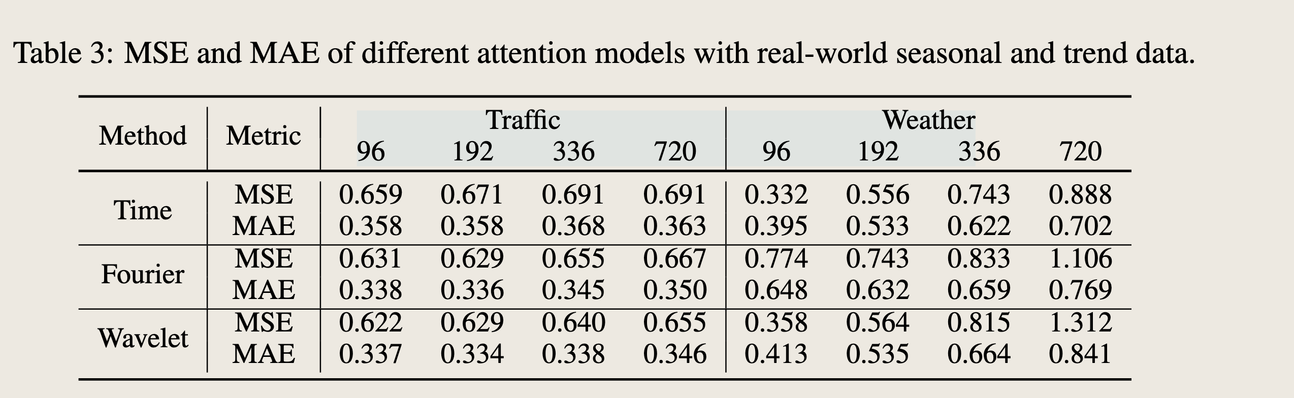
As an extension to experiments on synthetic data (Section 4), we also compare attention models on real-world datasets, and observe consistent results as on synthetic datasets. Note that for a fair comparison, we directly compare the attention models without additional components like decomposition blocks or additional learnable transformation kernels [4, 5]. We choose traffic dataset as data with seasonality and weather dataset as data with trend. As shown in Table 3, frequencydomain attention models demonstrate better performance with seasonal data, which aligns with our observations on synthetic datasets. For trend data, Fourier-attention models show larger errors compared with time and wavelet attention models, which is also consistent with our observations on synthetic datasets. Compared with the reported performance after seasonal-trend decomposition as in FEDformer [5] and Autoformer [4], the errors on seasonal data remain similar, while errors increase significantly on trend data. This emphasizes the importance of de-trending. We also replace Fourier attention with time or wavelet attention in TDformer in Section 6.4.

作为对合成数据实验（第4节）的扩展，我们还在真实世界数据集上比较了注意力模型，并观察到与合成数据集上一致的结果。

注意，为了公平比较，我们直接比较了注意力模型，而没有包含额外的组件，如分解块或额外的可学习变换核[4, 5]。

我们选择交通数据集作为具有季节性的数据，天气数据集作为具有趋势的数据。

如表3所示，频域注意力模型在季节性数据上表现出更好的性能，这与我们在合成数据集上的观察结果一致。

对于趋势数据，傅里叶注意力模型与时域和波形注意力模型相比显示出更大的误差，这也与我们在合成数据集上的观察结果一致。

与FEDformer[5]和Autoformer[4]中报告的经过季节-趋势分解后的性能相比，季节性数据上的误差保持相似，而趋势数据上的误差显著增加。这强调了去趋势的重要性。我们还在第6.4节中用时域或波形注意力替换了TDformer中的傅里叶注意力。

Main Results

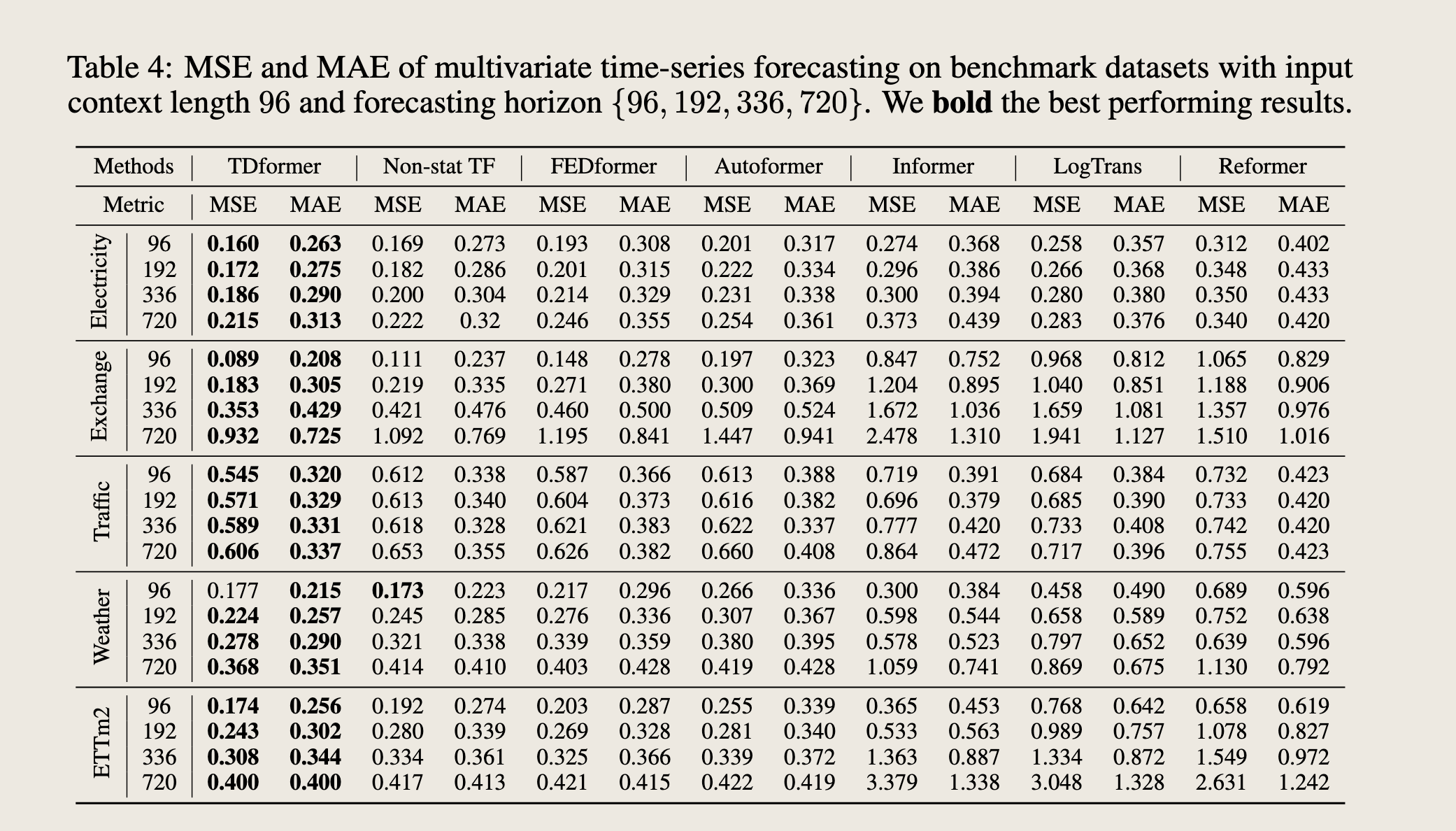
We compare TDformer with the state-of-the-art baselines and report on MSE and MAE in Table 4. TDformer consistently demonstrates better performance across different datasets and forecasting horizons. On average, TDformer reduces the MSE by 9.14% compared with Non-stationary Transformer and by 14.69% compared with FEDformer, and we attribute such improvement to our separate modeling of trend and seasonality with MLP and Fourier attention. As we mention in Remark 5, trend prediction of FEDformer and Non-stationary Transformer still come from attention modules, while TDformer decouples the modeling of trend and seasonality, and demonstrates better forecasting results. See Figure 1 for qualitative comparison.

我们将TDformer与最先进的基线模型进行了比较，并在表4中报告了MSE和MAE。TDformer在不同的数据集和预测范围上始终展现出更好的性能。平均而言，TDformer比非平稳Transformer的MSE降低了9.14%，比FEDformer降低了14.69%，我们将这种改进归因于我们使用MLP和傅里叶注意力分别对趋势和季节性进行建模。正如我们在备注5中提到的，FEDformer和非平稳Transformer的趋势预测仍然来自注意力模块，而TDformer将趋势和季节性的建模解耦，并展现出更好的预测结果。

新说法: TDformer decouples the modeling of trend and seasonality, and demonstrates better forecasting results 解耦建模

Ablation Study

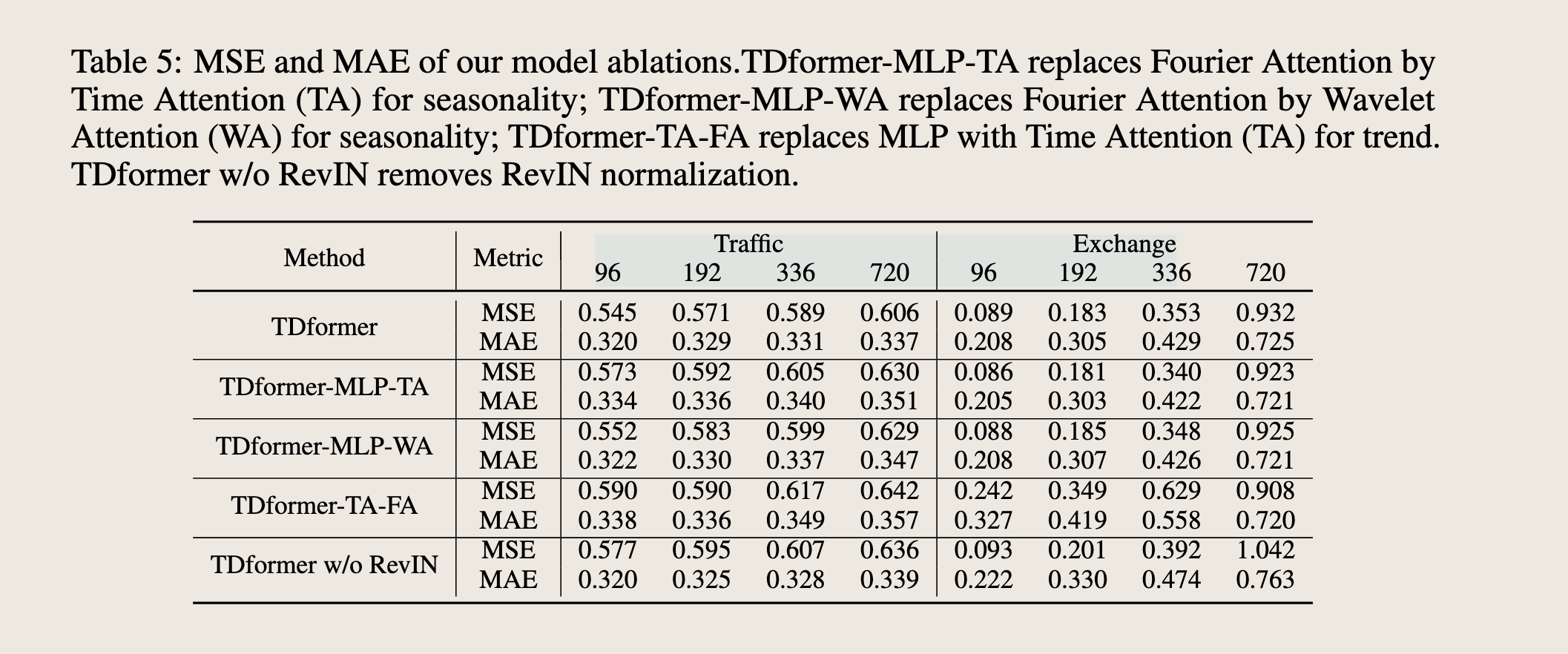
To separately understand the effect of trend and seasonal modules, we conducted ablation studies. TDformer-MLP-TA(WA) replaces Fourier attention with time (wavelet) attention for seasonality,and shows larger errors especially on seasonal data (traffic), as Fourier attention is more capable of capturing seasonality. Exchange data is mainly composed of trend, so different attention variants demonstrate similar performance with time attention being slightly better. We also replace MLP with time attention for trend (TDformer-TA-FA) and observe large errors, as attention models show inferior generalization ability on trend data. TDformer w/o RevIN removes RevIN normalization and displays larger errors, which shows the importance of normalization for non-stationary data.

为了分别理解趋势和季节性模块的效果，我们进行了消融研究。TDformer-MLP-TA(WA)用时域（小波）注意力替换了季节性部分的傅里叶注意力，并显示出更大的误差，特别是在季节性数据（交通）上，因为傅里叶注意力更能捕捉季节性。汇率数据主要由趋势组成，因此不同的注意力变体在时域注意力上表现相似，略好一些。我们还用时域注意力替换了趋势的MLP（TDformer-TA-FA），观察到大误差，因为注意力模型在趋势数据上显示出较差的泛化能力。TDformer w/o RevIN移除了RevIN归一化，并显示出更大的误差，这表明归一化对于非平稳数据的重要性。

Conclusion

In this work we are driven by better understanding the relationships and separate benefits of attention models in time, Fourier and wavelet domains.

We show that theoretically these three attention models are equivalent given linear assumptions.

(在线性注意力条件下的等价)

However, empirically due to the role of softmax, these models have respective benefits when applied to datasets with specific properties.

(softmax 的角色)

Moreover, all attention models show inferior generalizability on data with trend.

(注意力机制对于趋势性数据的拟合效果不好)

Based on these analyses of performance differences, we propose TDformer which separately models trend and seasonality with MLP and Fourier attention models after seasonal trend decomposition.

TDFormer = (trend->MLP) + (seasonal-> Fourier)

TDformer achieves state-of-the-art performance against current attention models on time-series forecasting benchmarks. In the future, we plan to explore more complicated models to predict trend (e.g., autoregressive models) and explore other seasonal-trend decomposition methods.

在这项工作中，我们旨在更好地理解时间域、傅里叶域和小波域中注意力模型的关系及其各自的优势。我们证明了从理论上讲，在满足线性假设的情况下，这三种注意力模型是等价的。然而，从经验上看，由于softmax的作用，这些模型在应用于具有特定属性的数据集时各自具有优势。此外，所有注意力模型在处理趋势数据时都显示出较差的泛化能力。基于这些性能差异分析，我们提出了TDformer，该模型在季节-趋势分解后，使用MLP和傅里叶注意力模型分别对趋势和季节性进行建模。TDformer在时间序列预测基准测试中取得了与当前注意力模型相比最先进的性能。未来，我们计划探索更复杂的模型来预测趋势（例如，自回归模型），并研究其他季节-趋势分解方法。

Appendix

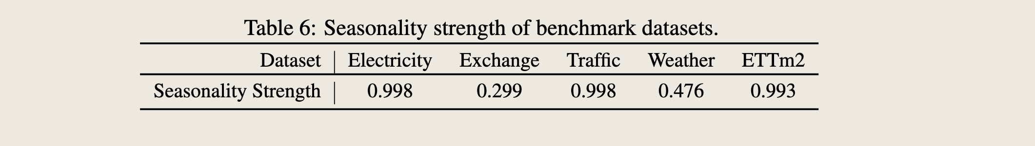
We first apply STL decomposition [14] for each dataset

where $T_t, S_t, R_t$ respectively represent the trend, seasonal and remainder component. For data with strong seasonality, the seasonal component would have much larger variation than the remainder component; while for data with little seasonality, the two variances should be similar. Therefore, we can quantify the strength of seasonality as

Following this equation, we summarize the seasonality strength of each dataset in Table 6. Electricity, traffic and ETTm2 are strongly seasonal data, while exchange rate and weather demonstrate less seasonality and more trend.

我们首先对每个数据集应用STL分解[14]

其中 $T_t, S_t, R_t$ 分别代表趋势、季节性和余项成分。对于具有强烈季节性的数据，季节性成分的变化将远大于余项成分；而对于季节性较小的数据，两个方差应该相似。因此，我们可以量化季节性强度为

根据这个方程，我们总结了表6中每个数据集的季节性强度。电力、交通和ETTm2是具有强烈季节性的数据，而汇率和天气显示出较少的季节性和更多的趋势。