summary
新建 summary.log 存储模型一次前向传播的过程
与 TimesNet
|
|
TimeMixer
|
|
这个参数相差的两级好离谱啊
| 模型 | 参数数量 | 参数大小 | 总内存占用 | 输入→输出 |
|---|---|---|---|---|
| TimesNet | 1,199,619,547 | 4798.48 MB | 6231.47 MB | [32,12,7]→[32,24,7] |
| TimeMixer | 190,313 | 0.76 MB | 81.10 MB | [16,96,7]→[16,720,7] |
forcast forward
|
|
- 输入
x_enc [32,96,7] x_mark_enc [32,96,4]
- 处理 self.__multi_scale_process_inputs 巨复杂 步进把
self.__multi_scale_process_inputs
第一句:
|
|
down_pool = AvgPool1d(kernel_size=(2,), stride=(2,), padding=(0,))
第二句:
|
|
[32,96,7] -> [32,7,96]
**第三句: **
|
|
存储原始值 [32,7,96]
|
|
同样存的原始值 [32,96,4]
第四句:
|
|
为下采样做准备?
|
|
for 循环, 这里 self.configs.down_sampling_layers = 3 ,在干嘛?
|
|
x_enc_ori.shape = [32,7,96]
down_pool AvgPool1d(kernel_size=(2,), stride=(2,), padding=(0,))
x_enc_sampling = torch.Size([32, 7, 48])
|
|
x_enc_sampling = [32, 7, 48]
permute = [32,48,7]
x_enc_sampling_list = list[tensor[32,48,7]]
知识点 1 Conv1d和AvgPool1d中,操作总是应用在最后一个维度
|
|
x_enc_sampling [32,7,48] 赋值给 x_enc_ori [32,7,48]
在对时间戳数据处理之前, 总结这里的形状变化, down_sampling_layers=3,则会产生以下尺度的序列:
| 下采样步骤 | x_enc_ori形状 | x_enc_sampling形状 | 添加到列表的形状 |
|---|---|---|---|
| 初始状态 | [32, 7, 96] | - | [32, 96, 7] |
| 第1次循环 | [32, 7, 96] | [32, 7, 48] | [32, 48, 7] |
| 第2次循环 | [32, 7, 48] | [32, 7, 24] | [32, 24, 7] |
| 第3次循环 | [32, 7, 24] | [32, 7, 12] | [32, 12, 7] |
看时间戳的处理
|
|
继续 true
|
|
-
第一个
::保留所有批次维度 -
::self.configs.down_sampling_window:在时间维度上每隔指定步长取样 -
最后一个
::保留所有特征维度 -
x_mark_enc_mark_ori形状为[32, 96, 4]
-
self.configs.down_sampling_window = 2
那么执行后:
- x_mark_sampling_list.append(…)添加形状为[32, 48, 4]的张量
- x_mark_enc_mark_ori更新为[32, 48, 4]
在下一次循环中:
- 再次应用
[:, ::2, :]操作 - 时间维度再次减半:[32, 48, 4] → [32, 24, 4]
- 依此类推…
与数据下采样的对比
| 数据下采样 | 时间特征下采样 |
|---|---|
| 使用AvgPool1d | 使用步长切片 |
| 计算时间步的平均值 | 直接抽取特定时间步 |
| 处理主要特征数据 | 处理时间编码信息 |
设计目的 : 确保时间特征与数据特征在各个尺度上保持一致
最后
|
|
将单一尺度的输入转换为多尺度表示列表。
输入序列长度为96,经过3次下采样(因子为2),则返回的多尺度表示为
x_enc 变为包含4个张量的列表:
- 原始尺度: [batch_size, 96, features] =[32,97,7]
- 第一级下采样: [batch_size, 48, features] = [32,48,7]
- 第二级下采样: [batch_size, 24, features] = [32,24,7]
- 第三级下采样: [batch_size, 12, features] = [32,12,7]
x_mark_enc 同理
- 0 = {Tensor: [32,96,4]}
- 1 = {Tensor: [32,96,7]}
- 2 = {Tensor: [32,24,4]}
- 3 = {Tensor: [32,12,4]}
这句话结束
|
|
得到 x_enc , x_mark_enc
x_enc 同理
- 0 = {Tensor: [32,96,7]}
- 1 = {Tensor: [32,48,7]}
- 2 = {Tensor: [32,24,7]}
- 3 = {Tensor: [32,12,7]}
**x_mark_enc **
- 0 = {Tensor: [32,96,4]}
- 1 = {Tensor: [32,48,4]}
- 2 = {Tensor: [32,24,4]}
- 3 = {Tensor: [32,12,4]}
看这个 for 循环
|
|
第一次 for 循环
i=0,x={Tensor: [32,96,7]},x_mark = {Tensor: [32,96,4]}
|
|
B=32,T=96,N=7
|
|
输入 : x={Tensor: [32,96,7]}
处理 : self.normalize_layers[i] = Normalize()
其中, self.normalize_layers = ModuleList( (0-3): 4 x Normalize() )
|
|
self.channel_independence = 1
|
|
输入 : x={Tensor: [32,96,7]}
.permute(0, 2, 1).contiguous() [32,7,96]
.reshape(B * N, T, 1) [32×7, 96, 1]
|
|
x_list[0] = [32×7, 96, 1]
|
|
x_mark = [32,96,4]
.repeat(N, 1, 1) [32×7,96,4]
|
|
x_mark_list[0] = [32×7,96,4]=[224,96,4]
|
|
一次 for 循环结束, 这里的一大段结束, 我们得到的是 x_list ,x_mark_list
x_list
- x_list[0] = [224,96,1]
- x_list[1] = [224,48,1]
- x_list[2] = [224,24,1]
- x_list[3] = [224,12,1]
x_mark_list
x_mark_list[0] = [224,96,4]
x_mark_list[1] = [224,48,4]
x_mark_list[2] = [224,24,4]
x_mark_list[3] = [224,12,4]
上面是标准化层
接下来是嵌入层
|
|
这里还是挺新奇的,因为之前看过的代码都是统一 norm,统一 EMbedding
|
|
输入:
- x_list[0] = [224,96,1]
- x_list[1] = [224,48,1]
- x_list[2] = [224,24,1]
- x_list[3] = [224,12,1]
self.pre_enc 很复杂,那步进把
self.pre_enc(x_list)
|
|
就一个函数,看起来并不复杂
pre_enc方法执行以下操作:
- 如果channel_independence=True:直接返回(x_list, None)
- 如果channel_independence=False:对每个时间序列进行序列分解(moving average分解或DFT分解),返回(季节性组件列表, 趋势组件列表)
嗯,原因:
打印的self.pre_enc内容看起来很复杂是因为Python的变量打印机制导致的。
当直接打印self.pre_enc而不是调用它时,Python不会显示方法的代码,而是显示一个绑定方法对象的引用,格式为:
|
|
这表示:
这是一个绑定到Model实例的方法
大括号内的内容是该方法所属的Model实例的完整表示
但是: self.pre_enc方法本身非常简单
如果想查看方法的实际代码,可以使用inspect模块
|
|
好了,没有疑问了,总结这里
这个方法的作用是在嵌入前进行预处理
如果设置了channel_independence=True,直接返回输入序列和None
如果channel_independence=False,则使用self.preprocess(一个移动平均分解器)将每个序列分解为两个组件(季节性和趋势),分别存入两个列表返回
注意哦,注意,这里返回的是列表
好了,下一部分:
|
|
根据是否有时间标记进行不同处理:
有时间标记时,将每个尺度的时间序列与对应的时间标记一起输入到嵌入层
无时间标记时,只使用时间序列数据
这里有 时间标记
|
|
输入 :
-
len(x_list[0]) = 4
-
x_list[0]
x_list[0][0].shape = [224,96,1]x_list[0][1].shape = [224,48,1]x_list[0][2].shape = [224,24,1]x_list[0][3].shape = [224,12,1]
-
x_mark_list
- x_mark_list[0] = [224,96,4]
- x_mark_list[1] = [224,48,4]
- x_mark_list[2] = [224,24,4]
- x_mark_list[3] = [224,12,4]
第一次遍历: i=0, x=[224,96,1], x_mark=[224,96,4]
|
|
步进
|
|
- 输入: x=[224,96,1], x_mark=[224,96,4]
- TokenEmbedding( (tokenConv): Conv1d(1, 16, kernel_size=(3,), stride=(1,), padding=(1,), bias=False, padding_mode=circular) )
- TimeFeatureEmbedding( (embed): Linear(in_features=4, out_features=16, bias=False) )
- 步进, self.value_embedding(x)
- x = self.tokenConv(x.permute(0, 2, 1)).transpose(1, 2)
- self.tokenConv = nn.Conv1d(in_channels=c_in, out_channels=d_model, kernel_size=3,padding=padding,padding_mode=‘circular’, bias=False)
- ⭐️ 1D卷积,卷的最后一个维度(这里是卷的最后一个维度,但变的是中间维度,conv初始化(输入通道数,输出通道数,kernelsize,stride,padding(最后的三个变量控制着形状的变化, 中间的维度控制输入通道数和输出通道数)))
- 这里 x= [224,96,1] → [224,96,16]
- 这里的 tokenEmbedding 有疑问
1 2 3 4 5 6 7def forward(self, x): # x原始形状: [batch_size, seq_len, c_in] # permute转换后: [batch_size, c_in, seq_len] x = self.tokenConv(x.permute(0, 2, 1)).transpose(1, 2) # tokenConv后: [batch_size, d_model, seq_len] # 最终输出: [batch_size, seq_len, d_model] return x输入: x = [32,96,1]
permute [32,1,96]
self.tokenConv = TokenEmbedding( (tokenConv): Conv1d(1, 16, kernel_size=(3,), stride=(1,), padding=(1,), bias=False, padding_mode=circular) )
哦,明白了,conv1d(输入通道数,输出通道数,kernel_size,stride,padding)
kernel_size,stride,padding 保证了形状的不变
但是通道数会变 从以前的 1 维嵌入到 16 维
这里想说,d_model=16(TimeMixer 特殊的)
①分尺度 Norm
②嵌入维度=16
随手补充: 1D 卷积 & 2D 卷积
1D卷积(nn.Conv1d) 1D卷积不处理中间维度,而是: 输入格式: [batch_size, channels, length] 卷积沿着最后一个维度(length)进行 中间维度(channels)作为卷积的通道数 2D卷积(nn.Conv2d) 2D卷积同样不处理中间维度: 输入格式: [batch_size, channels, height, width] 卷积沿着最后两个维度(height, width)进行 中间维度(channels)作为通道数 共同特点 无论是1D还是2D卷积: 通道维度总是在索引位置1 卷积操作在通道后的维度上进行 在处理序列前通常需要重排维度,使数据符合PyTorch的卷积期望格式 ===================================
tokenEmbedding做完了, 开始 temporalEmbedding
|
|
-
步进
-
return self.embed(x)
-
self.embed = nn.Linear(d_inp, d_model, bias=False)
-
self.embed = Linear(in_features=4, out_features=16, bias=False)
-
输入 [224,96,4] → [224,96,16]
-
Linear 处理最后一个维度
-
self.value_embedding(x) [224,96,1] → [224,96,16]
-
self.temporal_embedding(x_mark) [224,96,4] → [224,96,16]
-
x = self.value_embedding(x) + self.temporal_embedding(x_mark) 最后的输出 [224,96,16]
-
回到这里 enc_out = self.enc_embedding(x, x_mark) x [224,96,1] , x_mark [224,96,4] → enc_out [224,96,16]
|
|
enc_out_list[0].shape = [224,96,16]
所以这里的整个 for循环得到的结果
|
|
- enc_out_list[0].shape = [224,96,16]
- enc_out_list[1].shape = [224,48,16]
- enc_out_list[2].shape = [224,24,16]
- enc_out_list[3].shape = [224,12,16]
下一部分
|
|
- self.layer = 2
输入:
- enc_out_list[0].shape = [224,96,16]
- enc_out_list[1].shape = [224,48,16]
- enc_out_list[2].shape = [224,24,16]
- enc_out_list[3].shape = [224,12,16]
处理
self.pdm_blocks[0] → self.pdm_blocks[1] 这里有点复杂 步进
输出:
self.pdm_blocks[i]
类名: class PastDecomposableMixing(nn.Module):
|
|
forward 接收的输入: x_list
形状 :
- [0] [224,96,16]
- [1] [224,48,16]
- [2] [224,24,16]
- [3] [224,12,16]
|
|
初始化了一个列表
|
|
for循环
遍历的列表:
- [0] [224,96,16]
- [1] [224,48,16]
- [2] [224,24,16]
- [3] [224,12,16]
此时第一次循环 得到 的 x.shape = [224,96,16]
|
|
嗯,存储时间步长度 第一个循环得到的是 96
|
|
那其实可以直接说 length_list中的所有元素是 = [96,48,24,12]
现在的感觉就是 TimeMixer 对每个尺度分别处理
比如截止到目前为止
- Norm 是分尺度的
- EMbedding 是分尺度的
- 现在PDM 也是分尺度的
继续看后面吧
|
|
再次初始后两个列表,存储季节性成分和趋势性成分
- 你看现在传递的参数也是,传递的是列表(多尺度)(96,48,24,12)
|
|
输入: x_list
for 循环 遍历的列表:
- [0] [224,96,16]
- [1] [224,48,16]
- [2] [224,24,16]
- [3] [224,12,16]
得到 x 的形状 [224,96,16]
|
|
这里的作用是 趋势分解
输入: x [224,96,16]
处理: self.decompsition = series_decomp( (moving_avg): moving_avg((avg): AvgPool1d(kernel_size=(25,), stride=(1,), padding=(0,)))) ps. 这不就是复用的 Autoformer 的组件
输出:
- season.shape = []
- trend = [224,96,16]
|
|
这里不执行,所以也不看是在干嘛了
|
|
添加列表
season_list[0].shape = [224,16,96]
trend_list[0].shape = [224,16,96]
以上完成了第一次 for 循环
整个的 for 循环得到的东西
season_list & trend_list
season_list
- season_list[0] [224,16,96]
- season_list[1] [224,16,48]
- season_list[2] [224,16,24]
- season_list[3] [224,16,12]
trend_list
- trend_list[0] [224,16,96]
- trend_list[1] [224,16,48]
- trend_list[2] [224,16,24]
- trend_list[3] [224,16,12]
|
|
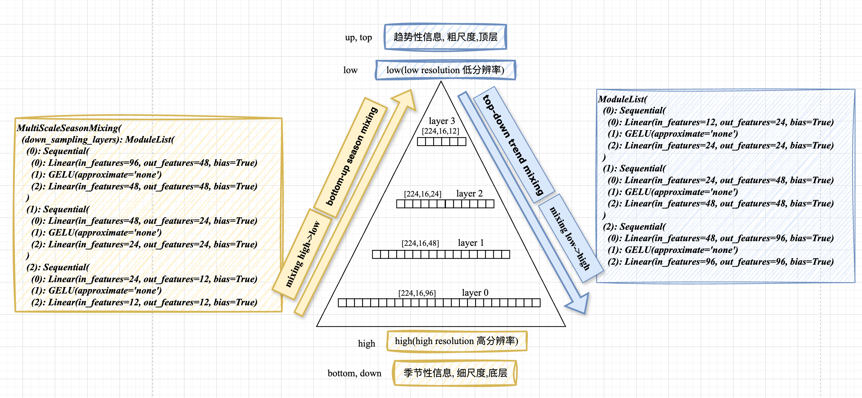
看注释: 自底向上的预测(季节性混合)
输入
- season_list[0] [224,16,96]
- season_list[1] [224,16,48]
- season_list[2] [224,16,24]
- season_list[3] [224,16,12]
处理 : self.mixing_multi_scale_season 的模型结构
|
|
- 输出:
步进 self.mixing_multi_scale_season
self.mixing_multi_scale_season
类名:
|
|
init 部分的模型
|
|
forward
|
|
接收的输入 season_list
- season_list[0] [224,16,96]
- season_list[1] [224,16,48]
- season_list[2] [224,16,24]
- season_list[3] [224,16,12]
整个forward 的部分代码并不复杂
|
|
out_high = [224,16,96]
|
|
out_low = [224,16,48]
|
|
输入: out_high = [224,16,96]
处理 permute(0, 2, 1) [224,96,16]
输出: out_season_list[0].shape = [224,96,16]
|
|
for 循环 len(season_list) = 4
i = 0
|
|
步进把,又是一个自定义类
这个步进不了
|
|
定义中使用的是ModelList 全是 pytorch 的自定义
- $\frac{96}{2^0} → \frac{96}{2^1} ,96 → 48$
- $\frac{96}{2^1} → \frac{96}{2^2},48→24$
- $\frac{96}{2^2} → \frac{96}{2^3},24→12$
实例化以后的结果:
|
|
configs.down_sampling_window 和 configs.down_sampling_layers是什么意思
-
多尺度季节性混合(Multi-Scale Season Mixing)
-
“自上而下”(高频到低频)特征融合
-
第一个线性层:将时间序列长度从
seq_len//(2^i)减少到seq_len//(2^(i+1)) -
GELU激活:增加非线性能力
-
第二个线性层:保持降采样后的长度不变,进一步学习特征表示
-
若seq_len=96,down_sampling_window=2,则创建:
- 层0:96→48
- 层1:48→24
- 层2:24→12
|
|
- 将高分辨率表示
out_high通过下采样网络转换为低分辨率表示out_low_res - 将下采样得到的表示与原始低分辨率表示
out_low相加融合 - 更新
out_high为融合后的表示 - 如果还有更低分辨率的层,更新
out_low为下一级别的季节性成分 - 将处理后的表示添加到输出列表
|
|
高频成分中的信息逐级传递到低频成分,使模型能够捕获并融合不同时间尺度上的季节性模式,增强对多周期模式的建模能力
懂了,开始吧
|
|
len(season_list) - 1 = 3
|
|
输入 : out_high.shape = [224,16,96]
处理: self.down_sampling_layers[0]:
|
|
输出: torch.Size([224, 16, 48])
|
|
输入: out_low.shape =[224,16,48] , out_low_res.shape=[224,16,48]
输出: out_low.shape = [224,16,48]
|
|
输入: out_low.shape = [224,16,48]
输出: out_high.shape = [224,16,48]
|
|
i + 2 = 2, len(season_list) - 1 = 3
满足条件,进入if 循环
|
|
输入: season_list[i + 2].shape = season_list[2].shape = [224,16,24]
输出: out_low.shape = [224,16,24]
|
|
输入: out_high.shape = torch.Size([224, 16, 48])
.permute(0, 2, 1) [224,48,16]
输出: out_season_list[0].shape = [224,48,16]
分析这里的 if 条件句
|
|
这个条件判断在执行以下操作:
-
检查是否存在更低分辨率的季节性分量:
-
当前正在处理season_list[i]和season_list[i+1]之间的融合
-
条件检查是否存在season_list[i+2](即下一级更低分辨率的分量)
-
-
准备下一轮迭代的输入:
-
如果存在更低分辨率分量,就将out_low更新为这个分量
-
如果不存在(已处理到最低分辨率),则保持当前的out_low不变
-
信息流动示例
假设有4个季节性分量(从高频到低频):
- 第0轮:融合分量0和1,然后准备下一轮使用分量2
- 第1轮:融合更新后的分量1和分量2,然后准备下一轮使用分量3
- 第2轮:融合更新后的分量2和分量3,此时没有更低分辨率分量可用
⭐️ 确保高频信息能够逐级传递到低频分量中,实现了不同时间尺度特征的有效融合。
⭐️ 在每轮结束时,处理后的特征通过permute(0, 2, 1)调整维度顺序后保存到结果列表。
懂了,最后总结一下文本图, 数据流动
|
|
- 信息级联传递:高频信息通过下采样逐级传递到低频
- 残差连接:out_low_res与每个尺度的原始分量相加
- 维度重排:返回时所有张量通过permute调整维度为[B,T,C]
- 多尺度融合:最终输出的每个尺度都包含了来自高频的信息
Okay 这句话执行结束
|
|
接收的输入 season_list
- season_list[0] [224,16,96]
- season_list[1] [224,16,48]
- season_list[2] [224,16,24]
- season_list[3] [224,16,12]
模型的输出: out_season_list 这里 d_model=16
- out_season_list[0] [224,96,16]
- out_season_list[1] [224,48,16]
- out_season_list[2] [224,24,16]
- out_season_list[3] [224,12,16]
处理的模型结构(见上)
下一句: 自顶向下的趋势性融合
|
|
输入, 传入 trend_list
- trend_list[0] [224,16,96]
- trend_list[1] [224,16,48]
- trend_list[2] [224,16,24]
- trend_list[3] [224,16,12]
输出, out_trend_list形状
对比: 季节性的融合 $96 -> 48 -> 24 -> 12$
趋势项
处理: self.mixing_multi_scale_trend
|
|
趋势的融合方向: $12->24->48->96$
步进 self.mixing_multi_scale_trend
类名: class MultiScaleTrendMixing(nn.Module):
forward:
|
|
输入: trend_list
- trend_list[0] [224,16,96]
- trend_list[1] [224,16,48]
- trend_list[2] [224,16,24]
- trend_list[3] [224,16,12]
|
|
复制操作,没啥说的
输出: trend_list_reverse形状
- trend_list_reverse[0] [224,16,96]
- trend_list_reverse[1] [224,16,48]
- trend_list_reverse[2] [224,16,24]
- trend_list_reverse[3] [224,16,12]
|
|
翻转操作,输出
- trend_list_reverse[0] [224,16,12]
- trend_list_reverse[1] [224,16,24]
- trend_list_reverse[2] [224,16,48]
- trend_list_reverse[3] [224,16,96]
|
|
out_low.shape = [224,16,12]
这里其实就是特征独立的处理,因为 批次和特征维度都合并了 32×7=224
|
|
out_high.shape = [224,16,24]
|
|
输入 out_low [224,16,12] permute(0,2,1) $->$ [224,12,16]
输出 : out_trend_list
复制 out_trend_list[0].shape = [224,12,16]
|
|
for 循环开始 合并趋势项
len(trend_list_reverse) - 1 = 3
|
|
输入 out_low.shape = [224,1612]
处理 self.up_sampling_layers[i]
|
|
输出: out_high_res.shape = torch.Size([224, 16, 24])
|
|
输入 out_high.shape = [224,16,24]
out_high_res.shape = [224,16,24]
输出 out_high.shape = [224,16,24]
这里有一点需要注意 你发现没,季节用的是卷积, 趋势用的是线性层
|
|
更新 out low为 [224,16,24]
|
|
同样的 if 条件句
|
|
这里不再赘述细节,意思就是为了融合
|
|
输入 out_trend_list
- out_trend_list[0] .shape = [224,12,16]
- out_trend_list[1] .shape = [224,24,16]
- out_trend_list[2] .shape = [224,12,16]
- out_trend_list[3] .shape = [224,96,16]
操作 .reverse()
输出 out_trend_list
- out_trend_list[0] .shape = [224,96,16]
- out_trend_list[1] .shape = [224,48,16]
- out_trend_list[2] .shape = [224,48,16]
- out_trend_list[3] .shape = [224,12,16]
下一句,返回结果
|
|
out_trend_list
- out_trend_list[0] .shape = [224,96,16]
- out_trend_list[1] .shape = [224,48,16]
- out_trend_list[2] .shape = [224,24,16]
- out_trend_list[3] .shape = [224,12,16]
|
|
好了,这句话执行完了,并返回结果
输入 trend_list
details
输入: trend_list trend_list[0] [224,16,96] trend_list[1] [224,16,48] trend_list[2] [224,16,24] trend_list[3] [224,16,12] ===================================
输出 self.mixing_multi_scale_trend
details
MultiScaleTrendMixing( (up_sampling_layers): ModuleList( (0): Sequential( (0): Linear(in_features=12, out_features=24, bias=True) (1): GELU(approximate='none') (2): Linear(in_features=24, out_features=24, bias=True) ) (1): Sequential( (0): Linear(in_features=24, out_features=48, bias=True) (1): GELU(approximate='none') (2): Linear(in_features=48, out_features=48, bias=True) ) (2): Sequential( (0): Linear(in_features=48, out_features=96, bias=True) (1): GELU(approximate='none') (2): Linear(in_features=96, out_features=96, bias=True) ===================================
处理 out_trend_list
details
输入: trend_list trend_list[0] [224,96,16] trend_list[1] [224,48,16] trend_list[2] [224,24,16] trend_list[3] [224,12,16] ===================================
弄明白了 开始下面咯
|
|
结果列表 TimeMixer 的处理单位是 列表
|
|
for 循环
输入:
-
x_list
- x_list[0] [224,96,16]
- x_list[1] [224,48,16]
- x_list[2] [224,24,16]
- x_list[3] [224,12,16]
-
out_season_list
- out_season_list[0] [224,96,16]
- out_season_list[1] [224,48,16]
- out_season_list[2] [224,24,16]
- out_season_list[3] [224,12,16]
-
out_trend_list
- out_trend_list[0] [224,96,16]
- out_trend_list[1] [224,48,16]
- out_trend_list[2] [224,24,16]
- out_trend_list[3] [224,12,16]
-
length_list
- [96,48,24,12]
第一次遍历 得到变量
- ori [224,96,16]
- out_season [224,96,16]
- out_trend [224,96,16]
- length 96
|
|
- 输入:
- out_season [224,96,16]
- out_trend [224,96,16]
- 输出 :
- out [224,96,16]
|
|
是否假设通道独立,这里的是 假设通道独立的,也就是 self.channel_independence=1
|
|
-
输入:
- out.shape [224,96,16]
- ori [224,96,16]
-
处理:
-
self.out_cross_layer
-
Sequential( (0): Linear(in_features=16, out_features=32, bias=True) (1): GELU(approximate=‘none’) (2): Linear(in_features=32, out_features=16, bias=True) )
-
结果:
- self.out_cross_layer(out).shape =[224,96,16]
-
补充这步的设计: 很像Transformer 中的FFN (d_model -> d_ff -> d_model ),但是 FFN 使用的 hiddensize=4×d_model
-
-
输出:
- out [224,96,16]
|
|
补充: out = ori + self.out_cross_layer(out)
多尺度信息融合:
- ori:原始时间序列编码表示 [224,96,16]
- out:季节性+趋势性混合后的表示 [224,96,16]
- self.out_cross_layer(out):对混合表示的非线性变换
self.out_cross_layer是一个前馈神经网络,包含:
- 第一个线性层:扩展特征维度(16→32)
- GELU激活:引入非线性变换
- 第二个线性层:压缩回原始维度(32→16)
最重要的还是要知道 这是模仿的 Transformer 的前馈网的设计
没什么想说的了 下一句吧
|
|
输入:
- out [224,96,16]
- length = 96
处理 :
- out[:, :length, :].shape = [224,96,16]
- out_list.append(out[:, :length, :])
- 得到输出: out_list[0] [224,96,16]
接下来就是 重复 for 循环
|
|
不再重复过程, 总结如下:
① 季节项 + 趋势项 比如 第一层 [224,96,16]
② self.out_cross_layer 模仿 Transformer的 FFN (d_model$->$d_ff$->$d_model) $[224,96,16]-> [224,96,32]-> [224,96,16]$
③ 添加到 out 输出列表, 需要注意的是 这里 处理来处理去 但是维度并没有变
- 最后返回 out_list
- out_list[0] [224,96,16]
- out_list[1] [224,48,16]
- out_list[2] [224,24,16]
- out_list[3] [224,12,16]
看点专业的说法
-
首先,代码遍历四个关键列表,对应每个时间尺度的数据:
-
ori: 原始输入特征 [B,T,C]
-
out_season: 经过自下而上(高频→低频)混合的季节性分量
-
out_trend: 经过自上而下(低频→高频)混合的趋势性分量 length: 原始序列长度
-
-
时间序列重组
- out = out_season + out_trend
- 将季节性分量和趋势性分量直接相加
- 这基于经典时间序列分解理论:时间序列 = 季节性 + 趋势性 + 残差
-
残差连接增强
- if self.channel_independence: out = ori + self.out_cross_layer(out)
- 当启用通道独立处理时,添加残差连接
- self.out_cross_layer: 一个小型FFN网络(d_model→d_ff→d_model)
- 作用:允许模型学习原始信号和分解重组信号间的非线性关系, 结构类似Transformer的FFN层,但应用在分解融合阶段
-
长度统一处理
- out_list.append(out[:, :length, :])
- 确保输出时间步与原始序列对齐
- 处理多尺度操作可能导致的长度变化
技术亮点
- 多尺度分解: 不同粒度时间尺度的特征提取
- 双向信息流: 季节性(底→上)与趋势性(顶→下)的互补流动
- 残差架构: 保留原始信息,缓解深度网络训练问题
行了,继续看代码把
以上执行完了 forcast $->$ self.pdm_blocks[0] (是,这个, 堆叠了两层 )
|
|
后面内容 见第二篇